The extrapolators in practice: nested-grid fidelity - Power-law decay of the buffer-stock consumption gap

The question, and the design¶

The theory pages prove how the consumption function behaves beyond any finite grid: above, the precautionary-saving gap dies as a power law with exponent $\min(1, \qup)$ (Theorem I); below, consumption approaches the maximal-MPC line at rate $\qdn = \rho$ (Theorem CE). This page reports the practical test: can a small grid, finished with the theory’s two tail extrapolators, reproduce the solution of a much larger grid — beyond the small grid’s own edges?

The design is a nested-grid protocol. A “truth” solution is computed on a deliberately enormous log grid ( $N_a = 6000$ points spanning $a \in [10^{-6}, 10^{8}]$ ). A small-grid solution is then computed on a strict subset of the same grid — $k = 1000$ points removed from each end, so every small-grid node is a truth node and all comparisons are node-aligned. The small solve is finished three ways: with the crude edge rules older solvers use (perfect-foresight above the top knot, $c = m$ below the bottom knot — “the rails”); with the two theory tails, participating in the solve itself; and with the tails attached only after a rails solve (evaluation-only), which isolates where the tails do their work. Two calibrations carry the two ends: an estimated high-school calibration (HS-mean — code id CAL-HS — $\qup = 0.38$ : the fat-gap top regime) and a $\psi \equiv 1$ zero-income-atom calibration (CE, $\rho = 2$ : the theorem-backed constraint end). Everything is deterministic and pre-registered; the run record and its verification battery live in the repository beside this page.

The tails are value-matched at the small grid’s knots and take their exponents from the theory alone — nothing is fitted to the truth:

\cFunc(m) = \bar \cFunc(m) - x_{\mathrm{knot}}\,(\wbar/\wbar_{\mathrm{knot}})^{-\min(1,\qup)} \quad\text{above;}\qquad \cFunc(m) = \bar\kappa\, m^e - K\,(m^e)^{1+\rho} \quad\text{below,}

(1)

with $\wbar = m - 1 + h$ the PF agent’s perfect-foresight total wealth (definition), $\bar\kappa = 1 - \pZero^{1/\rho}\ThornR$ the worst-atom maximal MPC (Prop C1), and $K$ pinned by continuity at the bottom knot.

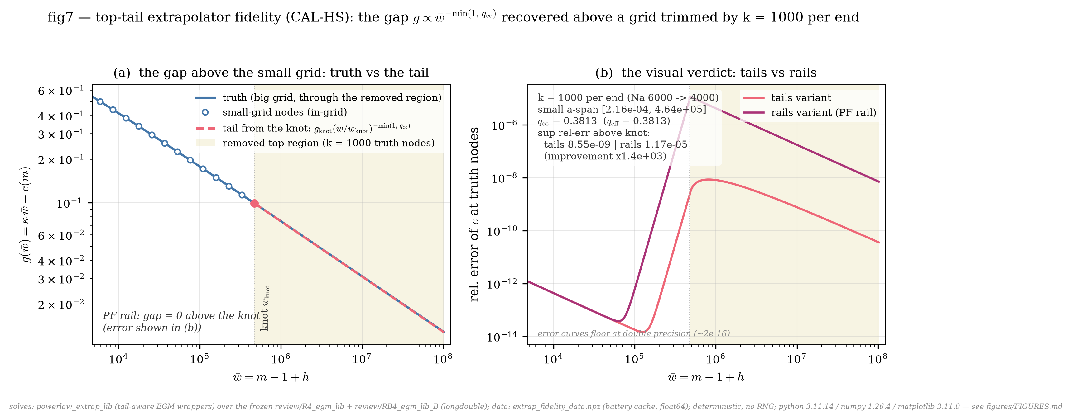
Two panels. Left, the precautionary gap above the small grid on log-log axes; the truth line runs through the removed region and the tail extrapolation lies on top of it. Right, the relative error of consumption at truth nodes; the tails curve sits about three decades below the rails curve everywhere above the knot. — Figure 1:**The top tail (HS-mean, $k = 1000$ per end).** Left: the gap $g(\wbar) = \kap\wbar - \cFunc(m)$ ; the tail leaves the small grid’s knot and lies on the truth through the entire removed region — two and a half decades of wealth the small grid never saw. Right: the visual verdict — sup relative error $8.6\times10^{-9}$ (tails) vs $1.2\times10^{-5}$ (perfect- foresight rail), a $\times 1{,}400$ improvement; the minimum per-decade improvement on the gap is $197\times$ .

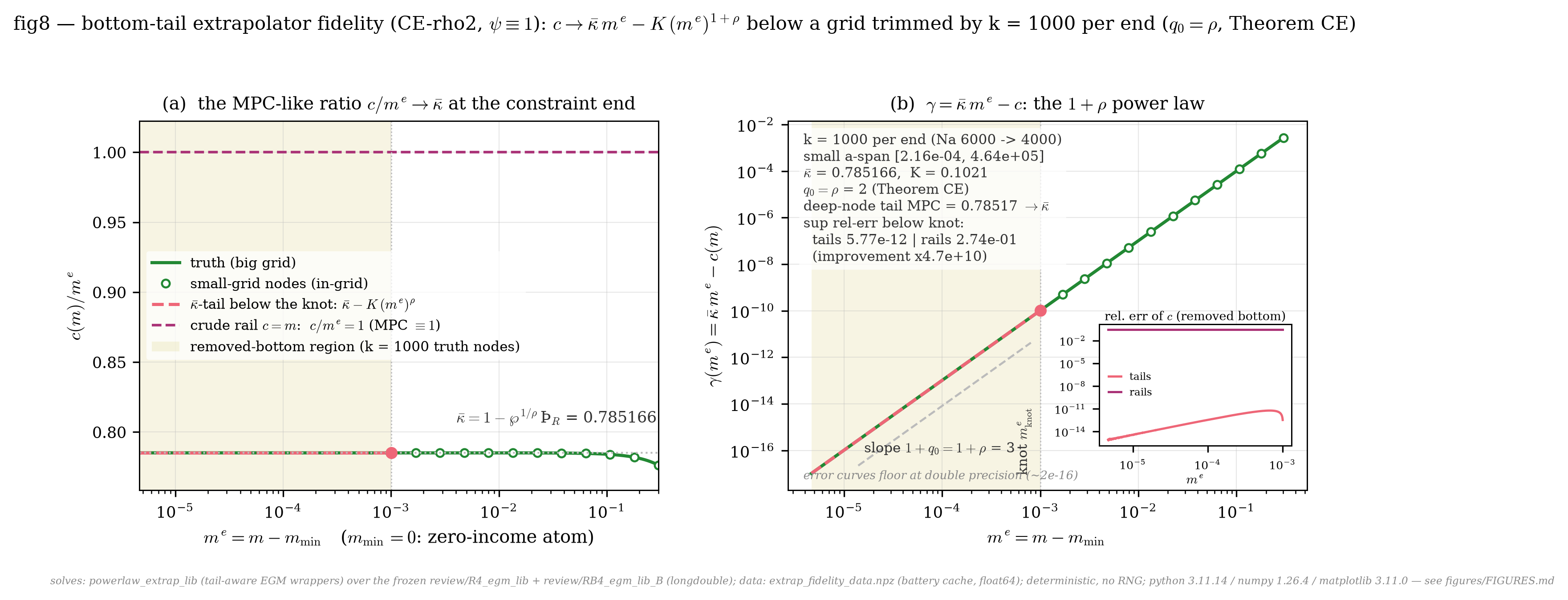
Two panels. Left, consumption divided by excess resources approaching kappa-bar at the constraint end, with the crude rail's horizontal line far above. Right, the gap to the maximal-MPC line on log-log axes riding a slope-three guide, with an inset showing the error curves eight decades apart. — Figure 2:**The bottom tail (CE, $\psi\equiv 1$ , $\rho = 2$ ; $k = 1000$ per end) — the first implementation of Theorem CE.** Left: $c/m^e \to \bar\kappa$ ; the crude $c = m$ rail asserts an MPC of 1 where the truth is $\bar\kappa = 0.785$ — a 27% consumption error the tail replaces with twelve digits of fidelity (sup relative error $5.8\times10^{-12}$ , a $\times 4.7\times10^{10}$ improvement); the tail’s MPC at the deepest node equals $\bar\kappa$ to 10^-6. Right: the gap $\gamma = \bar\kappa m^e - c$ rides the slope- $(1+\rho)$ guide exactly — the theorem’s power law, drawn by the data.

The finding that matters for solvers¶

An extrapolator plays two roles: it finishes the returned consumption function beyond the grid, and it participates inside the solve, because the Euler expectation evaluates next-period consumption at $\mNrmNxt = \Rcal a + \tranShkNxt$ , which overruns any realistic grid top whenever a large transitory draw meets a large asset node (and undershoots the bottom via the zero-income branch). The three-variant design separates the roles, and the answer is lopsided: the in-solve role carries almost all of the value. At the bottom, tails inside the solve beat evaluation-only tails by a factor $5.6\times10^{9}$ ; at the top, by $8.9\times10^{2}$ . A solver that only decorates its output function with a tail — leaving the crude rules inside the expectations — forfeits most of the benefit. This is the design requirement for any implementation: the tail must be wired into the solution loop.

What the gates say, honestly¶

The experiment ran under pre-registered gates, frozen before the first run. The headline fidelity gates passed as shown in the figures. Two audit-instrument clauses failed as artifacts of measurement floors — on the CE calibration the top-end gap is smaller than any solver’s convergence remnant can resolve ( $\qup \approx 49$ there, so $x/c \sim B/(\kap\wbar^2)$ ), and an adversarial verification pass proved the discrepancy equals the truth solve’s own convergence noise amplified by $c/x$ , while the tail’s amplitude matches the theory’s boundary value to $0.017\%$ . And one gate asked for more than nested grids can give: a trimmed grid solves a slightly different problem even at shared interior nodes, so in-grid agreement has a floor (measured: $6\times10^{-12}$ on CE, $6\times10^{-6}$ on HS-mean — the latter from a benign constrained-region channel that affects every variant equally). The full gate record, the amendment history, and the quantitative adjudication live with the battery in the repository.

Where this goes¶

The library behind this page mirrors the interface of HARK’s interpolation layer, and the measured numbers above are the evidence base for adding optional power-law extrapolation to HARK’s ConsIndShockModel (the top tail wires machinery already present in HARK PR #1782; the bottom $\bar\kappa$ -tail is new, and its theory is now complete: Theorem CE-ψ extends $\qdn = \rho$ to permanent shocks under a primitive contraction criterion, with the complementary regime characterized as a renewal problem — so the implementation regime-gates exactly as the theory states). The tails never touch the theory-verification batteries elsewhere in this corpus: the theorems are verified by solvers that know nothing of the laws they confirm, and this page’s truth solution is certified by extended-grid audits rather than by assumption.