The Power-Law Approach of the Consumption Function to its Perfect-Foresight Asymptote
The synthesis proof — the backward-induction spine, certified by its four rigor engines, illustrated on HAFiscal's estimated calibrations
0. The theorem in plain economics: precautionary saving as a discounted stream of premia, built backward (a reader’s guide)¶
The problem. The consumer solves the standard buffer-stock problem of BST — CRRA
utility, permanent and transitory income shocks, geometric discounting — whose complete
statement is the paper’s problem section.
This document works with the normalized problem under the assumptions listed in
§1 ((A1)–(A6), as itemized in statement.md §1; each element deep-linked
there to its anchor in the published BST draft).
The question. A very wealthy consumer facing labor-income risk behaves almost like a perfect-foresight consumer: income risk is trivial relative to wealth, so the precautionary motive nearly vanishes. How fast does it vanish as wealth grows? That rate matters computationally — every solution algorithm must assume something above its grid top — and theoretically: the buffer-stock canon proves the ratio version of the approach (BST’s limiting MPC bounds) but neither the level nor the rate (§3.3).
The answer in one sentence. Precautionary saving — the shortfall of consumption below the perfect-foresight rule — dies off as a POWER of wealth ((25), proved in §§5–6: Theorem 1, Paragraph; constructed transparently in §2) — the same functional family as the Pareto laws economists know from wealth, firm-size, and city-size distributions (Gabaix 1999, 2009, 2016) — with an exponent built from patience, returns, and growth ((2)), and (when ) a level (Theorem 1, (39)) that is nothing more exotic than a growing-perpetuity (Gordon) value.
The route. §1 states the model and the perfect-foresight benchmark; §2 builds the theorem by backward induction from a perfect-foresight resumption date — the presentation’s spine; §3 states the claim formally and places it in the literature; §§4–7 are the four rigor engines that certify the spine’s steps; §8 defines and measures the journey the spine describes; §9 cashes the theorem out computationally; §10 tallies the engines; §11 documents figures and reproduction.
The buffer-stock reading. The household’s buffer stock is its end-of-period assets . These households are impatient: absent the precautionary motive they would run their assets down to zero (under BST’s maintained zero-income event , which makes the natural borrowing limit zero; with they would borrow, toward the natural limit), so the assets they do hold are a buffer against the income risk. The buffer stock has a target : at , market resources are expected to reproduce themselves — at , the asset-side form of BST’s buffer-stock target (§3’s The target has the ψ-general form). In this document’s region the buffer stock stands far above and the household runs it down — normalized PF wealth descends at rate per period — while the behavior that would hold the buffer stock at its target (maintenance) is target-zone behavior, priced where the journey ends. What the theorem tracks along the descent is precautionary saving: , the eXtra saving relative to the perfect-foresight rule, which along the path satisfies — to leading order; the exact version, with its remainders sized, is §5’s one-step identity —
is the Kimball precautionary premium (KPP), and its dating deserves care. It is generated by next period’s shock (): prudence — Kimball (1990)'s — is evaluated where that shock will strike, tomorrow’s PF position (wealth , consumption ), and multiplies the consumption risk the MPC lets through, ; the product is , a function of today’s state only because tomorrow’s PF position is today’s state drifted once. It is then priced into today’s saving from one period away — whence its own , the same discount tomorrow’s expected saving carries. Unrolling the recursion, is the discounted stock of premia still to be provided along the journey, rung by rung: the KPP is always positive here (the forcing floor of §5, which is why ), and while the premium itself need not rise monotonically as wealth falls, the sum of the premia still to be provided grows with every backward step of the journey.
The scope of the asset-pricing resemblance — narrower than it first appears, and the rest of this document should be read accordingly. The resemblance is an asymptotic statement: it holds for LARGE , and its value is that it proves the power-law tail — the Gordon-perpetuity mechanics of §2 and the engines of §§4–6 are the payoff, and for that purpose the analogy is kept. It is NOT valid where the solution lives: the ergodic set (§8.1) sits at SMALL , and there the approximation fails on every count. The displayed formula for is only the limit — at smaller , especially near (bank balances near zero), the terms the derivation drops are no longer small and no closed form replaces them; even where the formula applies, the premium’s shape (a flow proportional to ) is nothing like a standard payoff stream; and in the limit the consumption function’s curvature becomes UNBOUNDED near the point where the liquidity constraint would bind (BST proves this), so no smooth pricing approximation can survive at the bottom. That is what necessitates numerical solution of the model in the ergodic region — the EGM methodology with the theorem’s tails (§9); the supplement why the standard asset-pricing toolbox does not replace it records the tool-by-tool case. The pointer: §2 gives the full and careful exposition, deriving the recursion and the premium’s formula by backward recursion from a final period at which risk ends, one newly risky period per step. Last, the premium’s positivity is a high-wealth theorem; the buffer-stock adjustment it finances is signed in general — a household whose buffer stock exceeds what it wants provides less, one short of it provides more. With that scope on the table: for the tail, (1) strongly resembles an asset-pricing recursion, and the Gordon-perpetuity mechanics below are the payoff of taking the resemblance seriously — there, and only there.
(Objects, for this section: — precautionary saving, the eXtra saving induced by precaution, the shortfall of consumption below the perfect-foresight rule. The PF-wealth-coordinate form is the gap ((7)); , with BST’s bank balances; §1 displays the definitions.)
None of this is posited: §2.3 derives the recursion, discount and adjustment included, from two Euler equations and a second-order expansion ((20)), and Lemma 5.1 ((29), §4) is its exact form (the translation box there spells out the precise discount and per-period flow). The adjustment is with PF total wealth — the Kimball precautionary premium (KPP) — the precautionary counterpart (Kimball 1990) of the Arrow–Pratt risk premium: absolute risk over PF wealth, hence tiny for the rich; (30), §3.4; the discounting per step is , with the state drifting down to (the wealth recursion (8)). Everything in the theorem is bookkeeping on this recursion, and §2.4 does the bookkeeping in a single geometric sum ((21)): the exponent is about which adjustments dominate the present value (near ones or far ones), the amplitude is a perpetuity value, and the trichotomy is Gordon-growth’s convergent / / divergent trichotomy.
What is ? (and why )¶
First the raw material — BST’s patience factors, written with the Old English thorn letter: is the absolute patience factor (the growth factor of perfect-foresight consumption); dividing by what consumption must keep up with gives return patience (RIC: ) and growth patience (GIC: — the impatience that makes wealth descend). §1 anchors each to its BST definition. Now two per-period log-rates, both familiar:
— the interest-minus-growth gap: how fast discounting compounds along the journey;
— the log growth-patience rate, NEGATIVE under GIC, so is the per-period descent rate: how fast an arbitrarily rich household runs its wealth down — its falls by the factor (about percent) per period — toward §8’s return region around the target.
Their ratio is the star of the theorem (at ; in general the root of (26)):
The intuition. The household’s state is ; perfect-foresight wealth is a function of it, — the same state relabeled into PF-wealth units (§1’s convention). The bar is BST’s upper-bound mark, not a mean: is not a constant. A change of units, not of position: no consumer ever “begins at ”. A wealthy household runs its buffer stock down, so its falls period by period; measured as , the fall is asymptotically exactly geometric — , dropping per period — which is exactly why the engines use these units. The journey ends not at a point but in §8’s return region around BST’s buffer-stock target : bounded shocks confine the recurrent range of wealth to a compact interval whose upper edge, in PF-wealth units, §8 computes as (8.1 How rarely is the tail visited? The dual (Kesten) root quantifies how rarely even that edge is visited from above). The time remaining from the current position is therefore periods — LOGARITHMIC in the current state (made exact by §5.2’s shells and Paragraph's shell-to-wealth conversion; later sections write , absorbing the edge’s additive constant into the amplitudes they track). Anything discounted exponentially in TIME therefore becomes a power law in WEALTH:
A power law in wealth is exponential discounting read on a logarithmic clock. (The same log-clock conversion generates the Pareto tails of the random-growth literature — there applied to cross-sections of cities and firms, here to a single household’s policy function.) So answers: by the time the big precautionary action arrives — near the target — how discounted is it, per unit of log-wealth?
(discounting beats the descent): faraway adjustments are negligible; the shortfall is dominated by the adjustment provided here and now, which is (Kimball). Realized exponent: 1 (Theorem 1).
(descent beats discounting): the shortfall is dominated by the large adjustments awaiting near the target, discounted back. Realized exponent: (Paragraph).
Hence : the shortfall is a sum of both components, and the slower-fading one wins asymptotically (Paragraph). And it can never fade faster than — a prudent consumer is always at least providing today’s adjustment (the floor on the forcing: stage-A Lemma 6.1 / stage-B Lemma B-6.1, restated with Lemma 5.1 in §4) — so the decay is a power law, not an exponential (Paragraph).
Permanent shocks make the descent NOISY (a random-walk component in log PF wealth). Runs of small permanent-income realizations () shrink the denominator of the normalized ratio and so inflate : excursions to high NORMALIZED perfect-foresight wealth are produced by bad income luck, not good — the household is income-poor and ratio-rich. Such runs weaken the effective descent toward the target, weakening the effective discounting and LOWERING below the deterministic ratio (§7, Theorem 2; the general- root solves (26)): for the estimated high-school calibration (HS-mean, §3.1), but ; at the college patience ceiling the deterministic ratio is , yet .
Half-lives, and an impatient billionaire. (2)'s ratio carries an inversion worth making explicit: more impatience means a smaller exponent — the gap fades more SLOWLY up the wealth ladder. There is no paradox. An impatient household converges quickly in time, and that is exactly why its gap dies slowly in wealth: even from the return region is only decades away, so the destination still shapes behavior far up the ladder. A nearly-patient household is the mirror image — the return temporally remote even at modest wealth, behavior that looks frictionless almost immediately. The per-quarter rates at the recurring calibrations (§3.1), converted to half-lives (, in years):
| calibration | descent (%/qtr) | half-life | discounting (%/qtr) | half-life | ratio |
|---|---|---|---|---|---|
| HS-mean | 1.25 | yr | 0.54 | yr | 0.43 |
| COL-TOP | 0.52 | yr | 0.51 | yr | 0.98 |
| GIC-CAP | 0.036 | yr | 0.51 | yr |
Standing at : the HS-mean household is years from the return region and still assigns it relevance weight ; the ceiling household is years away and assigns it 10-14 — economically invisible until the -tilt of (26) is priced in (: weight 10-1.5 — twelve orders of magnitude of Jensen). Hence: an impatient billionaire is still, at the margin, a buffer-stock consumer — a couple of decades from the return region, behavior visibly shaped by it — while a patient household of far more modest wealth already behaves as if frictionless. Households that converge fast in time are the ones whose gap decays slowly in wealth, and conversely. (The simplified capstone’s race appendix replays this race in slow motion — including a two-line lognormal reading of (26) that reproduces the exact roots of all four calibrations to a few parts in ten thousand.)
A characteristic root, and a saddle path. Economists solve linear rational-expectations models by finding the characteristic roots and discarding explosive solutions (Blanchard–Kahn). Equation (26) is exactly the characteristic equation of the linearized Euler dynamics in log wealth: the homogeneous solutions of the shortfall recursion are the powers with solving (26), and the exponent-detection theorem of §6 (Paragraph) is the corresponding stability selection — compensate by any wrong exponent and the transformed problem explodes or dies; only is the saddle path.
(For readers who do not live in linear rational-expectations models: the ‘homogeneous solutions’ are the family of alternative decay shapes the recursion tolerates on its own before economics is imposed; almost all of them either explode along the induction or violate a boundary requirement, and ‘the saddle path’ is the one shape that survives both tests. §2.4 performs this selection explicitly, with no linear-systems vocabulary required.)
The estimated calibrations. Three calibrations recur in the figures and numerical
checks. They arise in the context of the HAFiscal paper
(https://DiscFacEff) and the annuitized
return — whose product is invariant,
: the Euler equation, , , the GIC,
and the descent rate are all unchanged, while the budget side shifts
(, ,
, and rises). At the default
everything reduces to the model as written. Where mortality has
real consequences is the simulation phase — the ergodic distribution is
mortality-financed, and the two mortality channels pull the effective wealth support
in opposite directions (killing thins it; the annuity return fattens it — measured in
verify_sim_stability_checks.py) — which is why §8.1 and §9 invoke it and why the
simulation-phase analysis lives in the ergodic-coverage companion
(ergodic_coverage.md).
In the frozen verification code these appear
under their original identifiers CAL-HS, CAL-CTOP, CAL-CCAP, which are pinned instruments
and keep their names.
Translation table.
| in the mathematics | in economics |
|---|---|
| precautionary saving , in the PF-wealth coordinate the gap | the shortfall of consumption below the perfect-foresight (PF) rule |
| the forcing | the Kimball precautionary premium (KPP) — the coming period’s risk, priced today; the flow the recursion prices |
| the one-step identity (29) | strongly resembles an asset-pricing recursion: today = tomorrow + the adjustment |
| the backward unroll from ((21)) | the stock of premia still to be provided, accumulated over the remaining risky horizon — one newly risky period per backward step (§2.4) |
| the eigen-equation (26), root | the characteristic root: discounting speed ÷ descent speed |
| the slower-fading of “today’s adjustment” () vs “the discounted destination” () (Paragraph) | |
| the amplitude | the growing-perpetuity (Gordon) value of the adjustment stream (Theorem 1) |
| resonance | the Gordon knife-edge : value accrues linearly ⟹ the law (Paragraph) |
| the compactified boundary | “infinitely wealthy” treated like a steady state: change coordinates, then linearize there |
| shells | constant-percentage bands of PF wealth ≈ periods of the descent |
| the dual (Kesten) root (8.1 How rarely is the tail visited? The dual (Kesten) root) | the Pareto exponent of the wealth distribution’s random-growth machine |
1. Model, conditions, and the perfect-foresight benchmark¶
The model in full (each element deep-linked to its anchor in the published BST draft; the statement is BST’s, so a reader can check any piece against the source).
The symbol correspondence. This corpus (and its HARK consumers) writes relative risk aversion as and permanent income growth as ; BST’s published draft writes and for the same objects. Everything else is shared: (the absolute patience factor), , and (the limiting MPC bounds), (the zero-income probability), and (permanent and transitory shocks). One structural note: BST separates the transitory shock into the zero-income atom and the employed-state shock ( vs there); this corpus writes the all-in transitory shock as the single symbol — so the corpus’s is BST’s , and includes the atom.
Preferences. CRRA period utility with discount factor (BST, Setup). BST maintains , and the existence routing below inherits that; the decay arguments of §§3–5 use only once existence is in hand (assumption (A1) below).
The income process (Friedman–Muth; BST, Assumption assn-shocks, with the atom displayed at its transitory-shock definition). Permanent shocks : , supported on . Transitory shocks: income is zero with probability — the zero-income event, part of the assumption itself, not an optional garnish — and otherwise equals the employed-state shock (mean one, supported on a compact interval bounded away from zero, per BST) scaled by ; the all-in shock then satisfies and . Both shocks are bounded and mean-one in levels — this general statement, BST’s own (Assumption assn-shocks’s bounded-support requirement), is what every theory section below argues from; the equiprobable discretizations of lognormal shocks used by the figures are implementations consistent with it (bounded support excludes unbounded specifications but is consistent with all standard discretizations of unbounded distributions onto finite grids). One clause on what the atom buys: the results here do not all need — with existence routes through MST (2020) instead (below) — but is BST’s maintained specification, it is what the estimated calibrations use, and it is load-bearing for the form of WRIC, for the natural borrowing constraint (the discussion following Assumption assn-shocks), and for the MPC upper bound .
Budget transitions and normalization — the objects , , , , self-contained. BST’s within-period sequence, in levels: the consumer ends period holding assets (market resources minus consumption); those assets become next period’s kapital, — the same resources, renamed at the date they earn their return (BST’s ; without this definition the word “kapital” for date resources saved at would be mysterious); the return makes bank balances ; adding the period’s labor income gives market resources , from which consumption is chosen. Labor income is BST’s two-part process: permanent income grows by ( predictable growth, a mean-one permanent shock), and the period’s receipt is ( the mean-one transitory shock of (A3), zero-income event included). Dividing every level by permanent income — lowercase letters are these normalized ratios throughout, and the divisor below is exactly that renormalization crossing the period boundary — the problem is BST’s normalized Bellman equation: choose (as in the statement page) with transitions
where is end-of-period assets, next period’s kapital, next period’s bank balances — the returns realized on the kapital, the market-wealth leg of ((6)) — and next period’s transitory income. The first-order condition is BST’s normalized Euler equation, . At the growth-adjusted return is the constant and .
Human wealth and the perfect-foresight benchmark. Normalized human wealth — BST’s hNrm, the PDV of labor income including the current period’s — has infinite-horizon limit under FHWC (one line from BST’s finite-horizon definition). BST’s perfect-foresight consumption function is with limiting MPC , written in the decomposition its finite-horizon form displays — BST’s own (bank balances) — so in the variable displayed just below ((6)), and precautionary saving is — the object of the theorem. In the PF-wealth coordinate the same quantity is the gap , with — the engines’ object, because the PF drift is exactly multiplicative there (at zero gap (8) reads ); economics-facing prose keeps the household’s state . The one bookkeeping trap of the correspondence: ’s leading term is this period’s income, so the PF rule carries the -1; dropping it shifts by (checked to machine precision).
The perfect-foresight benchmark, displayed (the three defining displays the rest of the document consumes; the conditions named here carry BST anchors in the table below). Under GIC, RIC, and FHWC the normalized consumption function approaches its perfect-foresight asymptote from below:
where is BST’s human wealth — the PDV of labor income including the current period’s unit of it, which is why the rule (BST’s own, with from its limiting-MPC definition) carries the -1. The theorem is about the rate and form of that approach. Write
— the consumer’s total (human plus market) perfect-foresight wealth, viewed at the decision moment after this period’s returns have been realized on the kapital saved last period (): is BST’s bank balances ( at — market resources net of the unit of current income that already counts; BST’s own decomposition). The bar follows the convention BST itself states for — “the overbar signifies that will be an upper bound as we modify the problem to incorporate constraints and uncertainty; analogously, is the MPC’s lower bound” — bar = upper bound, underline = lower bound, matching ; itself is unused in BST, so no clash. One caution: bars so often mark CONSTANTS (means, bounds) that tempts a constant reading — it is not one: moves one-for-one with the state; after its definition, denotes its value — the engines’ coordinate. In this variable the PF rule is simply , and
— the same quantity as precautionary saving: .
The conditions, each with BST’s name, label, and live anchor:
| condition | BST label | statement | role in one clause |
|---|---|---|---|
| finite value of autarky | FVAC | value of always spending your permanent income is finite | |
| return impatience | RIC | PF consumption is a positive share of PF wealth () | |
| weak return impatience | WRIC | RIC weakened by the atom — enough for existence | |
| finite human wealth | FHWC | (i.e. ) | the PDV converges |
| growth impatience | GIC (-Raw) | normalized wealth drifts down when high | |
| strong growth impatience | GIC-Mod | delivers the target ; Jensen ⇒ strictly stronger than GIC for nondegenerate |
What the theorems maintain (Stage A / Stage B). Stage A (): (A1) CRRA ; (A2) constant ; (A3) the income process above with — i.i.d. , , , support with ; — BST’s maintained zero-income atom (Assumption assn-shocks) — is permitted throughout and is what the estimated calibrations use; (A4) FHWC; (A5) RIC; (A6) GIC(-Raw). Stage B adds i.i.d. , , , and FVAC. Unbounded-above is covered by the L4′ extension ( for some ) — the one deliberate departure from bounded support (8.1 How rarely is the tail visited? The dual (Kesten) root, item 3).
Existence, the atom, and the bounds. With the non-degenerate limiting solution exists by BST’s contraction theorems under WRIC + FVAC (the Boyd weighted-norm route — the atom is native to BST’s machinery); with one may instead invoke MST (2020) Theorem 2.2 (BST’s own remark maps the normalized problem into the MST framework as a special case). This routing is load-bearing and inherited by every proof in the program. The solution obeys BST’s MPC bounds with , and as — the ratio limit whose level-and-rate refinement is this paper (§3.3).
The target. Under WRIC + FVAC + GIC-Mod there is a unique target with at (BST’s buffer-stock-target theorem), computable from the implicit equation . An agent failing GIC-Mod has no target — the precise content behind the GIC-CAP name (§0); at the ceiling calibration even the mean log-drift is positive, so normalized wealth drifts up without bound (§8.1). Bounded support of the shocks (Assumption assn-shocks) is what makes the return region around (§8) a compact interval; BST’s own bounded-support discussion makes the same point — it is what permits the contraction-rate arguments characterizing the stable target to be made globally rather than only asymptotically.
The imported ladder (all PROVEN and review-hardened in stage_A_proof.md §§1–5 /
stage_B_proof.md §§B1–B3; statements only):
L0–L2′: existence/uniqueness/Euler (routing above); strictly increasing, strictly concave (Carroll–Kimball 1996); the sandwich ; non-increasing and convex; , .
L3 (level convergence): — two lines from the gap equation, and not stated anywhere in the published canon (§3.3).
The exact PF-wealth recursion, with the a.s. excursion bound (Cor 3.2):
(Today’s saving is invested: the term relaxes tomorrow’s budget — remember it for the translation box in §4.)
Lemma A5: (26) has a unique positive root; is convex with .
(Lemma 5.1 and Corollary 5.2 — the exact one-step law and its monotone comparison sandwich, the induction invariant that certifies the spine — complete the imported ladder; they are stated in §4, where they are consumed.)
2. The spine: equation (1) by backward induction from ¶
The theorem’s construction order is backward. Fix a date at which the consumer faces —
or believes she faces — no further uncertainty, so that she resumes the perfect-foresight
rule from on; every earlier period faces the transitory risk. Stepping backward from
, each step adds one newly risky period, and §0’s discounted stock of premia
grows exactly as the pricing recursion (1) says it should. This section
constructs that recursion — the discount, the drift, and the adjustment all derived, not
posited — and unrolls it to the published constants. The setting is the Stage-A world
(: transitory shocks only, per §1); §2.6 records that the
construction is -general. Everything here is exact to leading order in , with
the dropped terms itemized in §2.5 and certified by the rigor engines of §§4–7 (the map:
(EQ-1) ↦ Lemma 5.1’s (29) and Cor 5.2’s sandwich; the unrolled sum ↦ §5’s shells; the
truncation at the log-clock exit ↦ §8’s return region). The spine’s named battery is
verify_eq1_backward_checks.py (§11), which implements the backward iteration exactly and
checks every displayed constant.
2.1 The terminal date, and the two identities that do all the work¶
The normalized transitory-only model of §1: CRRA , ; period budget/transition with , (FHWC), , , bounded . The normalized Euler operator is
Perfect-foresight (PF) objects ((5), (6)): with (, RIC), , and perfect-foresight total wealth ( BST’s bank balances, §1),
(The -recursion is (8) at zero gap: and the bracket vanishes identically by ; .)
Two elementary identities carry the whole derivation:
(I1) is the PF Euler equation itself: with PF consumption growth . (I2) is RIC bookkeeping: and .
The terminal assumption. At date the agent faces — or believes she faces — no further uncertainty, and therefore behaves according to the PF rule from on:
Before she faces the transitory risk. We iterate backward.
2.2 One step back (): the doubly-differentiated Euler subtraction¶
(The section title unpacked: write the Euler equation twice — once for the agent who knows next period’s shock will be at its mean, once for the agent facing the risk — Taylor-expand both to second order in the shock, and subtract. Everything zeroth- and first-order cancels; the surviving second-order term is the premium, and the surviving first-order-in-the-gap terms are the recursion.)
Write the two Euler equations at — the agent who KNOWS (she is the PF agent, ), and the agent who faces the risk ():
Let be tomorrow’s perfect-foresight market resources (its PF wealth is ), and abbreviate . The stochastic argument is .
Expand (EE-sto) to second order in around — the double differentiation of the spine’s name. With :
so, taking expectations, the first-order term dies because , and at the second term of dies because exactly:
Expand the remaining argument in (small; verified ex post) and subtract (EE-det). On the left, . The zeroth-order terms cancel by (EE-det) — this is where “the first-order terms disappear”: what survives is first order in and second order in :
Both sides in CRRA, evaluated on the PF ray (, ): , . Divide through by and use (I1) twice ():
By (I2), the bracket is exactly — the messy marginal-utility coefficients collapse — and:
This is the time- version of equation (1): a pure power law in with exponent 1 and an explicit amplitude. Its reading: is the Kimball precautionary premium in marginal-utility units (prudence times the risk the MPC passes through); dividing by the local marginal-utility gradient and discounting turns it into consumption units. Note that (19) equals — the adjustment priced at tomorrow’s PF wealth , then discounted one period at the interest-minus-growth factor . The bracket’s feedback term has its own economics: consuming less today banks more for tomorrow, which lowers tomorrow’s marginal utility and so offsets part of today’s precautionary wedge; identity (I2) says this offset is exactly what converts the naive discount into the risk-free one.
2.3 The induction step: equation (1) exactly, with its discount and adjustment derived¶
Now step to (and generically to any ), assuming the shortfall exists and is small in the bootstrap sense of §2.5 (it is: it was just constructed, of order ). Repeat the subtraction. Three — not two — pieces survive, all first order in the small quantities or second order in :
the feedback (as in §2.2): — today’s shortfall banks assets;
the injection (as in §2.2): ; the piece now reads — two orders in below the term (§2.5), dropped;
the propagation — new: tomorrow’s consumer is herself short of HER PF rule, so contributes , the continuation shortfall priced in marginal utility. ( to leading order; the Jensen correction is second order, §2.5.)
The same division by , the same (I1)–(I2) collapse, and — writing everything in PF-wealth coordinates, with the argument naming the coordinate, 's PF wealth — the recursion is
— shortfall today = (discounted at ) shortfall tomorrow at the deterministically drifted PF wealth , plus the discounted adjustment. This is §0’s pricing recursion (1) — the expectation there evaluated at its certainty equivalent, the drifted PF wealth — with every term now derived: the discount is the interest-minus-growth factor (not , not — identities (I1)–(I2) do the conversion into consumption units along the PF ray); the state drifts by per step (the wealth recursion (8)); and the flow is the Kimball precautionary premium of §3.4, with identically in this leading-order form — exactly the forcing limit (30) of the rigorous lemma. The rigorous counterpart is Lemma 5.1’s exact identity (29) (§4), , whose monotone comparison form (31)/(32) is (EQ-1) with the honest PF-wealth-drift slack; the remainders , collect exactly the terms §2.5 drops.
2.4 Unrolling backward: the Gordon trichotomy with the published constants¶
Iterate (EQ-1) backward from , steps, using :
Every claim of the theorem set is now a statement about this geometric sum — the Gordon growing-perpetuity trichotomy, with per-step ratio : each backward step, the adjustment grows by (the state has drifted down one rung) while discounting compounds by . This is §0’s stock of premia literally accumulating, one newly risky period at a time.
(a) : the perpetuity converges. gives
exactly (27) — the number Theorem I (Theorem 1) certifies as the boundary value (39). The gap is : the realized exponent is .
(b) : , the resonance. Every term contributes equally ( each). The sum does not run forever: after steps (the log-clock, (3); , NEGATIVE under GIC, so is the per-period descent rate) the drifted PF wealth has descended to the buffer-stock body and the high-PF-wealth adjustment formula no longer applies. Arithmetic accumulation over the journey:
exactly the resonance constant of (40). The knife-edge factor of (25) is nothing but arithmetic accumulation.
(c) : the perpetuity diverges — the far adjustments dominate. The sum is dominated by its LAST terms: adjustments provided near the end of the descent, at moderate PF wealth, discounted back over the whole journey. Truncating at the log-clock exit :
recovering (26)'s exponent at :
((2)). Equivalently and more structurally: the homogeneous solutions of (EQ-1)
are the self-similar modes with per-step multiplier
; self-consistency — the eigen-equation (26) — and modes
shallower than die out under backward iteration (), modes steeper
explode (), so the far tail is the slower of {the particular
injection mode, the homogeneous mode}: exponent , which is
(25) — the mode selection §6’s Theorem γ-T (Paragraph) certifies. Two
features of the sharp statements fall out for free: the amplitude in this regime is set
where the truncation happens — in the body, NOT locally at large : the maintenance
end of the journey, where the descent lands on the hold-at-target (target-zone) behavior of
§0’s reading, is for literally what sets the amplitude (why this case
has no local closed-form ; cf. t1_amplitude_supplement.md) — and the
backward steps land on the geometric lattice , i.e. an arithmetic
lattice of spacing in , which is the origin of the log-periodic factor
in the sharp form (statement.md’s Theorems A2/B2 lattice sum
with period ; the envelope is Paragraph).
(Concretely: feed a trial power-law shape through one backward step of the recursion with the forcing switched off. It comes back as the same shape multiplied by a constant factor that depends on the trial exponent: shallower-than-critical shapes come back smaller — they die out along the induction — while steeper ones come back larger — they explode. ‘Mode’ means nothing more than a shape the step maps to a multiple of itself.)
The finite-horizon corollary, for free. At any finite distance from the sum (21) is finite, so the gap is exactly-order at ANY finite horizon regardless of — the Method of Moderation’s “the slope is exactly 1 at finite horizon; only in the limit” (§9).
2.5 Why the constants come out exact: the order count¶
The expansion parameter is NOT : it is the size of the shock relative to PF wealth. Fix the -distribution and let grow. With and the bootstrap class, the dropped terms are:
Table 1:Error bookkeeping: every dropped term is subleading in
| dropped term | size relative to the kept terms |
|---|---|
| (third moment) | |
| in (gap curvature) | — an order below even |
| linearization curvature | |
| Jensen in propagation () | relative |
| evaluation-point shifts ( vs ) | relative |
All are or better relative to the retained terms — for a FIXED specification; the constants are NOT uniform over the family, in whose limit becomes unbounded near the constraint kink (BST) and the threshold below grows accordingly; nothing in this section is claimed for small — uniformly on over the bootstrap class — the same inventory Lemma 5.1 certifies as factors with ((29), §4). So the truncation at second order is not an approximation that happens to be decent: every neglected term is subleading in , which is why the construction lands on the exact (27), the exact resonance constant, and the exact eigen-root — the same constants the rigorous chain certifies (Theorem 1, Paragraph). “Second order around ” is the whole story at the top because prudence () is the lowest-order derivative that sees risk at all, and scaling demotes everything beyond it.
What the backward telling does not prove — and where the rigor engines take over: that the true infinite-horizon is the limit of this construction with uniform control (value-iteration convergence with the stated uniformity is part of the rigorous chain); that the dropped remainders cannot conspire (Lemma 5.1’s , bounds plus the comparison engine (31)/(32) handle exactly this; §4); and the sharp forms at (Theorems A2/B2 and the γ-engine statements of §6).
2.6 The spine is -general (pointer)¶
Nothing above is special to . The W3 spike (eq1_backward_psi_spike.md;
battery verify_eq1_psi_spike_checks.py, ALL PASS, cross-run byte-identical) re-runs the
doubly-differentiated subtraction with permanent shocks and finds three exact
-cancellations: (K1) the Euler weight exactly absorbs the
-dependence of next-period consumption’s level along the PF ray; (K2) the
-weighted innovation mean is exactly zero, so the first-order term dies
-generally and the adjustment keeps its Kimball form with
((42)); (K3) the asset-feedback coefficient is -invariant, so the
discount stays exactly . The mode multiplier becomes
; self-consistency
is the eigen-equation (26) exactly, and the unrolled
amplitude at is (28) exactly. §7 states the rigorous Stage-B
results; the derivation itself is not imported.
3. The formal claim and its place in the literature¶
3.1 The claim¶
(A reading guide for the displays that follow: they are one claim specialized three ways. The exponent is always the smaller of 1 and q_∞. When q_∞ exceeds 1 an amplitude LEVEL exists — the Gordon value, with its ψ-general form. Exactly at q_∞ = 1 the level is replaced by the logarithmic resonance form. Below 1 the amplitude is set in the body, and a log-periodic wobble can ride on it.)
§2 built the approach; here is its formal statement. An infinite-horizon consumer with CRRA utility (coefficient ) faces the Friedman–Muth income process of §1 — i.i.d. mean-one permanent shocks and transitory shocks , whose specification includes the zero-income atom — under the buffer-stock conditions GIC, RIC, and FHWC ((A1)–(A6), §1). The statement lives in the perfect-foresight wealth coordinate (6), with the gap of (7). The gap decays as a power law with exponent ,
where is the unique positive root of the eigen-equation
with sharp closed-form amplitudes. At ,
and at , (at : ; (40)). At the sharp form carries a periodic factor (Theorems A2/B2 of the original chain; the envelope is Paragraph). Figure 1 shows the object and the three slopes.
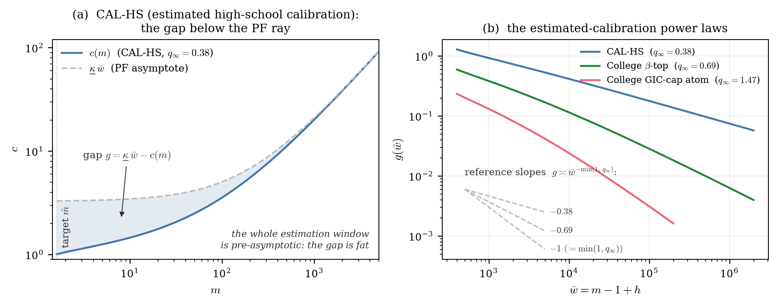
Figure 1:The gap and its power law. Left: and the PF asymptote for HS-mean, on (log–log, from the target up): the two rules visibly merge — at the right edge human wealth ( for this calibration) is of PF total wealth — with the gap shaded. Right: vs on log–log axes for the three estimated calibrations, with dashed reference slopes .
How to read this figure. Left: the true consumption function and the perfect-foresight line, plotted to high enough wealth (, where human wealth is of PF total wealth) that the two visibly merge — the shaded wedge between them (precautionary saving ) is what the theorem is about. Right: log–log paper, where a power law is a straight line — exactly as in the Pareto plots economists draw for wealth or city-size distributions. The slope is the exponent . A shallower line means prudence fades more slowly with PF wealth: for HS-mean (slope -0.38) the precautionary motive remains quantitatively alive far up the wealth ladder, while at the patience ceiling (slope -1) it dies off at the fastest admissible rate.
Why measured slopes bend: the purification rate. At any finite depth the plotted lines
are not yet perfectly straight, and the theorem also says how fast they straighten. To
leading order the gap is not one decaying thing but a mixture of two dying components:
the homogeneous component of the pricing recursion (1), fading at
the eigen-root rate of (26) per -fold of , and the component
continually re-fed by the KPP forcing, fading at rate 1 per -fold (the premium
itself shrinks like ). The asymptotic power law belongs to whichever component
dies more slowly — that is the in the theorem — and the other is a
contaminant still visibly present at any realistic depth. Because the ratio of two
exponentials decays at the difference of their rates, the mixture purifies at the
mode-gap rate : the contaminant’s share shrinks by the factor
per -fold of , so is the number of -folds one must climb to
shrink the measured slope’s error by a factor of . At COL-TOP (, mode
gap 0.31) a unit of purification costs -folds — a climb in
PF wealth — which is why the fitted deep slope there is still shy of even
at (digits and fit windows in figures/FIGURES.md), while at HS-mean
(, mode gap 0.62) the same unit costs only -folds and
the fitted slope agrees with to . The same arithmetic is the speed limit
on any tail attached at a finite grid top: what a knot-based extrapolation measures at
the top node is the mixture, not the asymptote, and the measured slope’s excess over the
true exponent dies off no faster than per -fold beyond the knot. Near
the resonance the mode gap closes and purification stalls — only the
logarithmic factor separates the components — so there the knot’s measured slope stays
informative arbitrarily far out.
All computational figures use calibrations estimated in the HAFiscal paper (full
provenance in figures/FIGURES.md; discount factors are survival-adjusted, as there):
HS-mean, based on the estimated parameters of a representative high-school-educated
household (); COL-TOP, the most patient college-educated type as estimated
(the top of the estimated discount-factor distribution, ); and
GIC-CAP, the college patience ceiling ():
its is capped a hair below the boundary at which BST’s raw growth impatience
condition (GIC) would fail; at that patience,
BST’s Strong Growth Impatience condition
(GIC-Mod, §1) — whose failure marks the frontier beyond which an agent is so
patient that no target level of wealth exists and wealth grows without bound — has already
failed (§8.1). The three span the trichotomy: the two estimated calibrations
live in the regime (exponent itself), the patience ceiling in the
regime (exponent 1). Two clearly-labeled auxiliary calibrations appear only where
a regime cannot be exhibited at estimated patience (the exact-resonance panel; the resolved
periodic-factor inset).
3.2 Situating the result: function-approach, not distribution-tail¶
A reader who knows the modern heavy-tails literature in economics should be told immediately what this theorem is not. The celebrated power laws of Toda (2014), Benhabib–Bisin–Zhu (2011, 2015), Stachurski–Toda (2019), Beare–Toda (2022), and Gouin-Bonenfant–Toda (2023) concern the cross-sectional distribution of the level of wealth (or income, or firm size): Pareto tails of a stationary distribution, with the tail exponent solving a Kesten-type root equation for the forward dynamics. This paper’s object is different in kind: it is the consumption function itself — a policy function, not a distribution — and the claim is that approaches the perfect-foresight solution according to a power-law decay process in the individual decision-maker’s wealth as that wealth goes to infinity.
The distinction is sharp, not cosmetic. In the transitory-only model (,
bounded ) under GIC, the ergodic distribution of wealth has compact support —
there is no Pareto tail of any kind, a fact whose econ-packaged form is precisely
Stachurski–Toda’s (2019) impossibility theorem (risk-free saving + constant with
⇒ wealth inherits the income tail). Yet the consumption gap is exactly a power
law. Formally, the two literatures’ root equations are Mellin duals: the
distributional-tail equation may fail to have any root (it
does fail at ) while the primal equation (26) always has one — the level
is what saves it. The full kinship map (which constructions could and could not
transport a distributional-tail theorem to the primal gap) is alt_proof_econlit.md §6; the
one live bridge candidate (a geometrically-killed running maximum, nearest published
statement Beare–Seo–Toda 2022) is recorded there with its four blocking gaps. Section
8.1 How rarely is the tail visited? The dual (Kesten) root develops the dual root explicitly — with the estimated calibrations’ numbers — for readers
meeting it for the first time.
(Mellin duality, in one sentence: the Mellin transform is the change of variables to log wealth, which turns multiplying wealth by a factor into adding a step — under it the two literatures’ root equations are the same equation seen from the two sides, which is why one side can have a closed form while the other does not.)
3.3 The near-miss frontier: what the literature proves, what is new¶
The buffer-stock/income-fluctuation canon comes remarkably close to this theorem without stating it. (Throughout, lemmas of this program are cited by their source labels — L0, L1, …, with primes marking strengthened variants such as L2′; γ-prefixed labels belong to the compactified engine of §5.) What is published:
| known result | source | what it gives | what it lacks |
|---|---|---|---|
| ratio limit | BST (Limiting MPC Bounds); MST (2020) Prop 2.5; Ma–Toda (2021) Thm 2.3; Ma–Toda (2022) Thm 2.6 | no level, no rate | |
| derivative limit | BST (in-text squeeze; not a numbered theorem — flagged) | eventually monotone | no rate |
| rich-end growth | BST (Asymptotic Consumption Growth Factors) | behavior PF benchmark | a limit, not a rate |
| sign: approach from below | Carroll–Kimball (1996) concavity; Leland (1968)/Sandmo (1970) | — | |
| level convergence | nowhere (verified sweep, 2026-07-07) | — | proven here (L3; §1’s imported ladder) |
| the rate + amplitudes | nowhere | — | the theorem |
Two hygiene notes from the verified survey: Ma–Toda (2022) states explicitly that it does not characterize the rate; and the Euler-iteration existence canon (Li–Stachurski 2014, MST 2020 Assumption 2.3, Ma–Toda 2021) requires , which fails at the zero-income atom (CRRA when ) — so existence for the model with the atom routes through BST’s WRIC/FVAC machinery, not through that canon (§1).
3.4 The forcing is the Kimball precautionary premium (KPP)¶
The engine below runs on a one-step recursion whose inhomogeneous term is, to leading order, — economically, ( times) the Kimball precautionary premium (KPP) — the precautionary counterpart (Kimball 1990) of the Arrow–Pratt risk premium — for the coming period’s normalized income noise, evaluated at PF-wealth scale : Kimball’s (1990) form with CRRA relative prudence . Its sign in this region (the gap is positive: uncertainty depresses consumption below the PF line) is Leland (1968)/Sandmo (1970); its small-risk quadratic template is Pratt (1964); its consumption interpretation is Drèze–Modigliani (1972).
4. Rigor engine I: the induction invariant¶
Every step of the spine leaned on a leading-order recursion; the four engines now make it
rigorous, and the first is the induction invariant itself: the exact form of (EQ-1).
Lemma 5.1 rewrites the Euler equation exactly in gap form — (EQ-1) ↦ (29) — with the
spine’s leading-order adjustment replaced by the exact forcing (two-sided
bounds; limit (30) the of §2.3), and with everything §2.5’s table drops
carried honestly as the certified remainder weights .
Corollary 5.2 is the sandwich that makes §2.4’s unrolling honest: its two branches
(31)/(32) are (EQ-1) with the stochastic PF-wealth step bracketed by
its worst-case displacement , so the backward iteration proceeds without knowing
the realized path. Both are PROVEN and review-hardened in stage_A_proof.md §§1–5 /
stage_B_proof.md §§B1–B3 (statements only, completing §1’s imported ladder):
The one-step gap identity (Lemma 5.1) — the Euler equation, exactly rewritten in gap form for :
with the precautionary forcing, two-sided bounds , the limit
and remainders , . The remainders , collect everything the leading-order reading drops: the evaluation-point shifts and linearization curvature of the exact gap identity. They obey and , so they vanish as : every neglected effect is one order higher in than the terms kept (the error-bookkeeping table of Table 1 in §2.5 itemizes them).
The monotone comparison form (Cor 5.2) — the workhorse the compactified engine consumes:
(‘Monotone comparison’ just means: bracket the random one-step map between its two deterministic extremes — the step with the most favorable shock and the step with the least favorable one. Each bracket can be iterated on its own, giving an upper and a lower staircase that squeeze the true solution between them; every later engine consumes those two one-sided iterations.)
an upper and a lower comparison,
Economic reading of (31)–(32): today’s gap = (discounted at ) tomorrow’s gap at the deterministically-shrunk PF wealth , plus the discounted adjustment , the coming period’s risk priced today — the buffer-stock journey, one rung at a time.
Formally, the sandwich (31)–(32) strongly resembles a pricing recursion — shortfall = discount × continuation shortfall + adjustment, with the Kimball adjustment as the flow (§0’s buffer-stock reading). Readers who internalize this one line can predict every result in §§5–8 by asking the corresponding asset-pricing question: does the perpetuity converge? what happens at ? which adjustments carry the value?
5. Rigor engine II: the unrolling made uniform — the compactified boundary fixed point¶
§2.4 stepped backward one period at a time and truncated the sum at the log-clock exit; making that honest for the infinite-horizon policy — uniformly in the number of backward steps, with the stochastic drift and the -remainders live — is this engine’s job. Its device is a change of coordinates under which the whole backward journey fits on one compact picture: the shells of §5.2 are §2.4’s backward steps seen in the state space (one shell = one rung of the descent = one tick of the log-clock), and the boundary point is “ seen from the state space” — the place where infinitely many backward steps accumulate, compactified so that “take the limit” becomes “evaluate at the boundary”. The scalar equation at that boundary (§5.4) is §2.4’s geometric sum, resummed as a fixed point.
(Proof bodies: alt_proof_compactified.md §§1–3, refuter-reviewed (RF1/RF2, zero broken);
labels below are that document’s. One notational bridge: that document writes the trial
exponent as ; here it is (and precautionary saving is , §0).)
5.1 The coordinate, and “assuming the power law in the limit” as a choice of units¶
Map . The half-line becomes , and infinite wealth becomes the finite boundary point — adjoin it. (This is the one-dimensional Poincaré-compactification chart of dynamical systems; Dumortier–Llibre–Artés 2006, ch. 5 — decorative ancestry, no theorem of theirs is consumed.) Then choose units that embed the conjectured power law: the compensated gap
(The idea in one line: adjoin ‘wealth equals infinity’ to the state space as an honest boundary point, so that ‘take the limit as wealth grows’ becomes ‘evaluate at the boundary point’ — statements about limits become statements about continuity at a place the analysis can stand on.)
“Assume the power law holds in the limit” is thereby demoted from a hypothesis to a choice of coordinates: nothing is assumed — §6’s Theorem II (6. Rigor engine III: the trichotomy certified — Theorem II, resonance, and the sharp forms) shows the compactified problem itself detects the right exponent ( has a finite nonzero boundary behavior only at ). Figure 2 gives the geometry.
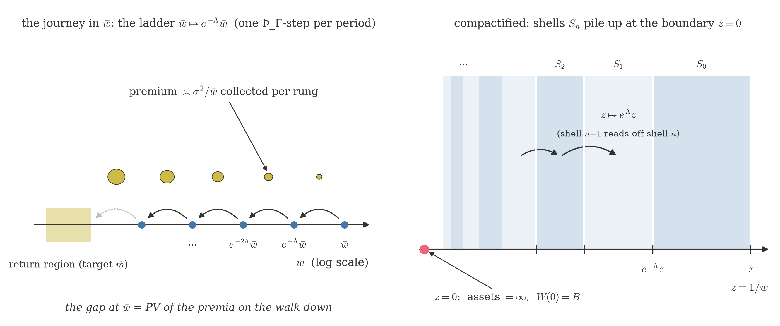
Figure 2:The ladder and the compactified shells. Left: in wealth space the recursion marches down toward the return region around the target, providing an adjustment per rung. Right: in the shells accumulate at the boundary point (“PF total wealth ”); the referred point points away from the boundary, so the recursion at shell always reads off the already-controlled shell .
How to read this figure. Left: economics. A household richer than its buffer-stock target saves less than income-plus-interest, so its wealth-to-income ratio drifts down about percent per period (the GIC drift); each rung of the descent calls for an adjustment proportional to . Right: the same journey after the change of variables , which puts “infinitely wealthy” ON the page as the point — the way a phase diagram puts a steady state on the page. The arrows show why the argument is not circular: the recursion always maps a point toward the region where the solution is already controlled, so information flows from known territory to the boundary, never from an assumption about the boundary.
5.2 The shell equation¶
Partition into geometric shells (log-width ), accumulating at the boundary; enlarge each by the constant — the exact fixed point of the one-step displacement map (the unique with ) — so the referred point of every in shell lands exactly in shell (Lemma γ0; no band slack, no self-reference: the map points away from the boundary, so the recursion at shell always reads off the already-controlled shell ). In these units the imported sandwich (31)–(32) becomes the shell equation (Lemma γ1).
(‘Referred point’ means: the wealth level the one-step map sends the current level to. The enlargement constant is chosen precisely so that this image always lands a full shell down — never straddling a shell boundary — and that non-straddling is what lets the induction walk down one shell at a time without circular reasoning.)
For compensation , its upper and lower branches read
with boundary-continuous coefficients: the multiplier (at — an algebraic identity via ) and the forcing , whose boundary limit at is by (30), consumed rate-free. There is also the exact identity
which is never used to produce a limit — only to evaluate one after it exists.
5.3 The two core lemmas (the entire engine — 76 lines in the source)¶
Lemma γ2 (boundedness). is bounded on the compactified domain. Idea: iterate the sup of (35) inward shell by shell; with and bounded forcing, the sup recursion with is trapped by . Self-contained — Theorem A1 is not imported.
(Intuition for boundedness: a contraction factor strictly below one means each shell’s worst case is pulled toward the injection’s scale instead of compounding on itself; the summability of the perturbations says their total lifetime effect is finite — too weak to undo the contraction.)
Lemma γ3 (boundary stability — the engine). For two-sided shell recursions with and : both and of equal . Proof (the four lines): let ; passing to the limsup in the sup-recursion gives , so ; the mirrored inf recursion gives ; closes it.
(The proof in words: the recursion says each shell’s worst case is at most a contraction factor strictly below one times the previous shell’s worst case, plus a bounded injection. Worst cases therefore cannot ratchet upward: in the limit the largest recurring value M satisfies M ≤ λM + F̄, which pins M ≤ F̄/(1−λ). Running the same argument from below on the best cases gives a matching floor, and the two one-sided bounds meet at the Gordon value.)
5.4 Theorem I (the owner’s one number): the boundary value at ¶
Proof (assembled). γ2 gives boundedness; γ0/γ1 put the shell sequences in γ3’s hypotheses ( by boundary continuity of the coefficients, by (30), the factors are the with because is geometric); γ3 forces , i.e. the limit exists. Only then is (37) passed to the limit (dominated convergence; , uniformly, a.s.-and-bounded), which yields (38) — the order matters, and is what makes the argument non-circular (refuter-verified explicitly, RF1 §audit-1).
(Unpacking the chain for readers who have not memorized the labels: γ2 says the compensated gap never explodes on any shell — its worst cases stay bounded; γ0 and γ1 are housekeeping — the injections converge and the weights settle; γ3 then converts ‘bounded, with settling inputs’ into an actual limit; and the limit is the Gordon value. Each lemma is stated and proved just above.)
This is the promised punchline: at the boundary point “PF wealth ” the entire Euler equation degenerates to one linear scalar equation, and the finite number representing the exact limit is its unique solution. The unrolled form is the geometric resolvent — the same number every other proof in the program computes by its own route (§10). (Rigor record: the source suite measures the deep-tail match to the closed form at 0.9% with the predicted approach rate fitted to 0.597 vs 0.6.) Figure 3 shows both faces: panel (a) the GIC-CAP calibration (, Stage B), where the boundary value exists and the boundary equation pins it — but the approach outruns reachable PF wealth ( at the top of the estimation grid, 0.91 even at the grid top; the knife-edge window of §9); panel (b) a labeled illustration calibration where the same convergence completes in-window (match 1.3%; inset slope -0.598 vs -0.6).
The Gordon-growth reading of is §2.4’s unrolling, resummed: adjustment growth per rung of the descent, discounting per period, convergence exactly when — the Gordon condition “discount rate exceeds growth rate”, which is (case (a) of §2.4, (21)) — and : the exact closed form of Theorem I, reached there by backward accumulation and here as a boundary fixed point. The entire theorem can be read as: the precautionary shortfall of the wealthy is the Gordon value of their future adjustments.
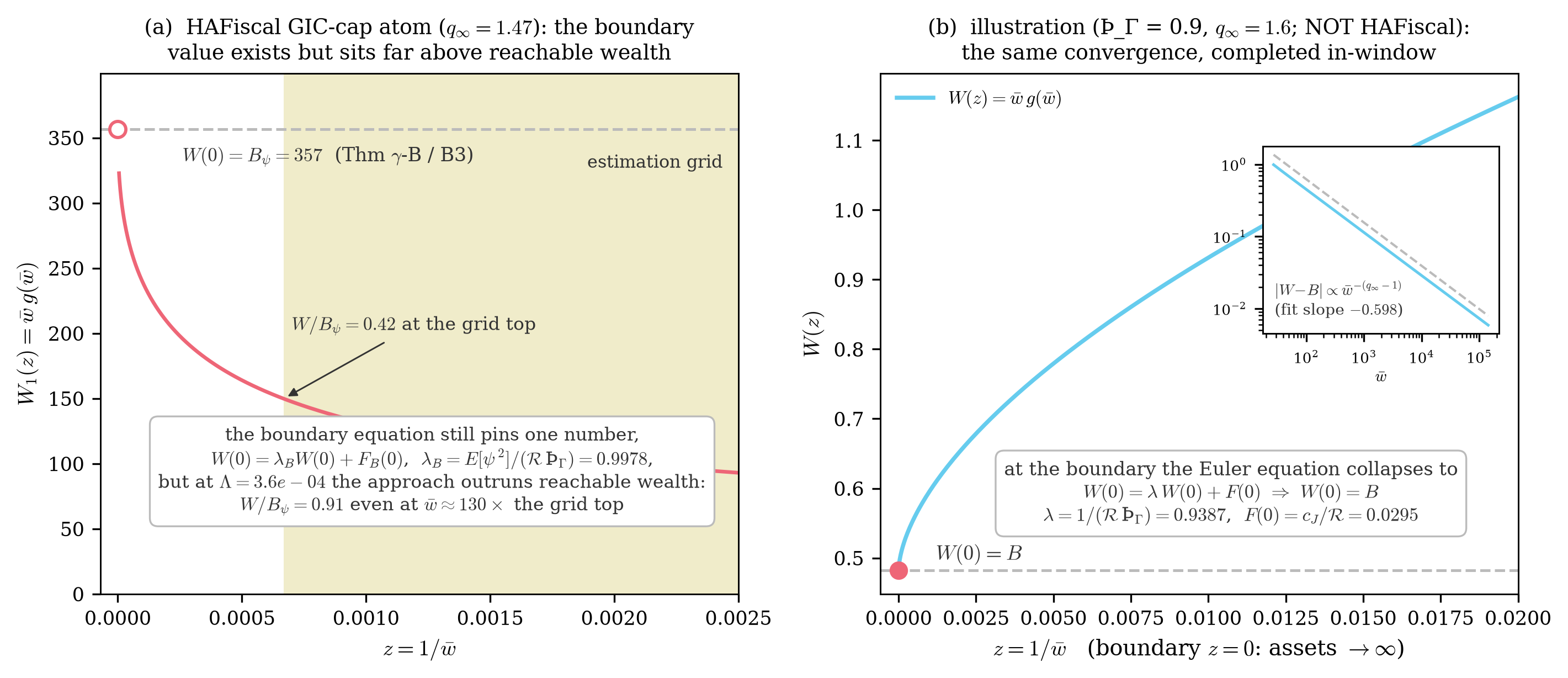
Figure 3:The compactified boundary value. (a) The GIC-CAP calibration: the boundary equation pins , but at the approach outruns reachable PF wealth. (b) An illustration calibration (, ; not HAFiscal): the same convergence, completed in-window.
How to read this figure. The vertical axis is PF wealth × shortfall — call it the amplitude. If the shortfall truly behaves like , this product levels off at the constant ; moving leftward along the horizontal axis () means growing richer. Panel (b), the labeled illustration economy: the amplitude does level off, at exactly the closed-form perpetuity value — the marked dot at the boundary. Panel (a), the patience-ceiling calibration GIC-CAP: the same leveling is provably underway, but its destination () lies far above anything visible on the computational grid (shaded region) — at the grid top the amplitude has covered only 42% of the way. Practical moral: on any feasible grid, a fitted constant would badly understate ; the top-of-grid boundary condition should use the closed form, not a fit.
6. Rigor engine III: the trichotomy certified — Theorem II, resonance, and the sharp forms¶
§2.4 classified the unrolled sum by its per-step ratio ; Theorem II certifies that classification at the boundary, including the two members the spine could only sketch — the resonance constant, and the sharp forms in which §2.4(c)'s backward lattice becomes rigorous shell/renewal bookkeeping.
Test a trial decay exponent against the recursion: a mode is multiplied, per backward step, by the discount and by the drift-rescaling (the state contracts to , so a steeper trial exponent harvests a larger rescaling). The two effects exactly offset when — that balance is what defines — and for any other trial exponent the mismatch compounds at the rate per step: modes shallower than die out under backward iteration (), modes steeper explode (), which is why the fixed point selects (general : — so “boundary multiplier ” is literally Lemma A5’s eigen-equation (26)). Everything in the theorem is the elementary classification of the shell recursion by :
| regime | multiplier | forcing | boundary behavior | result |
|---|---|---|---|---|
| , | contracting fixed point — one number | Theorem I: | ||
| , | linear escape — a slope, not a value | Theorem γ-R | ||
| , | geometrically | multiplier exactly 1, fading forcing — a limit set | γ-C |
In Gordon-growth language the three rows are §2.4’s trichotomy, certified: the convergent perpetuity (a), the knife-edge whose linear accrual is the law (b), and the divergent case (c), in which the “value” is dominated by the latest, largest adjustments — the journey’s end near the target, whose imprint is the periodic fine structure.
Resonance (Theorem γ-R; PROVEN). At (), the shell recursion is with : by the perturbed Stolz–Cesàro lemma (γ-R1), ; converting shells to PF wealth (),
(Stolz–Cesàro is the discrete l’Hôpital rule: when the per-step increments of a sequence settle to a constant, the running average settles to the same constant. At resonance the discounting and the descent cancel exactly, so every backward step contributes the SAME undiscounted amount — after n steps the sum is about n times that amount, and since the journey takes about log-wealth-many steps, a factor of log wealth survives in the law. That is the entire origin of the knife-edge logarithm.)
— the sharp resonance constant of Theorem B-res’s corollary, re-proven in a few lines (measured to 0.07% in the source suite). Figure 4(b) exhibits it at the resonance patience level of the College fundamentals ( root-found so exactly, sitting between the most patient estimated College type (COL-TOP) and the patience ceiling (GIC-CAP)): grows linearly in the tilted shell index with per-step increment (deepest measured increment 1.101 vs theory 1.113). This is a knife-edge, not a neighborhood: the theorem is a fixed- statement, and the crossover to it is non-uniform on any window with (Remarks 3.4/4.1 of the source; the two deliberately-registered FAILs of the source’s falsifier suite live exactly there, adjudicated honest by two refuter panels).
: the boundary is a circle, not a point (γ-C; envelope PROVEN, sharp form imported). At the map shifts log PF wealth by exactly , so it leaves unchanged the position within the multiplicative cycle: the fractional part . In log PF wealth the dynamics repeat with period , so what matters asymptotically is the position modulo — a circle of circumference rather than a single boundary point. PF-wealth levels sharing the same position in the cycle (equal log PF wealth modulo ) form a family that the shell recursion maps to itself; on each such family the recursion neither contracts nor expands (its multiplier is exactly 1) while its forcing fades geometrically. Proven self-contained here: the two-sided envelope converges to a bounded positive limit set , (γ-C1), and the period-by-period smoothing of the position-in-the-cycle distribution contributed by the continuous part of the shock is geometrically summable (γ-C2). Upgrading to convergence separately at each position of the cycle needs a uniform bound on how much the limit can vary under small shifts of the position (a modulus of continuity in the cycle variable) — GAP-γ-equicont, honestly open for this engine (it is L8/L9 doubling territory); the sharp statement — , with the log-periodic factor, whose non-constancy is now directly measured (first resolved tone: amplitude at ) — is Theorem A2 of the original chain, imported. Figure 4(c) makes the practical point sharply: at HS-mean’s estimated patience () the periodic component provably has no effect at any attainable precision: its total amplitude — the oscillation of the log-periodic factor — satisfies , far below any numerical floor. That is, the boundary circle collapses numerically to a point — which is exactly why a constant-coefficient power-law extrapolant works in the HAFiscal/HARK code; the inset shows the one calibration in the program with a numerically resolved tone (, amplitude , correlation 0.9999 between the measured wiggle and its predicted position in the cycle) — the honest evidence that the circle is real.
(Where the circle comes from: below the resonance the journey’s endgame depends on where within one descent-step the log-clock lands — its fractional part — and positions that differ by a whole step are equivalent. ‘Position modulo one step’ is a point on a circle, and the log-periodic wobble in the law is the shadow that circle casts.)
(Plainly, what is missing: a proof that the wobble of the compensated gap within a single shell cannot speed up without bound as the shells accumulate — ‘equicontinuity’ is the analysts’ name for that uniform-wobble bound, and the cited doubling estimates are the standard tool that delivers it. No economic content is in doubt; only this uniformity step is open for this engine.)
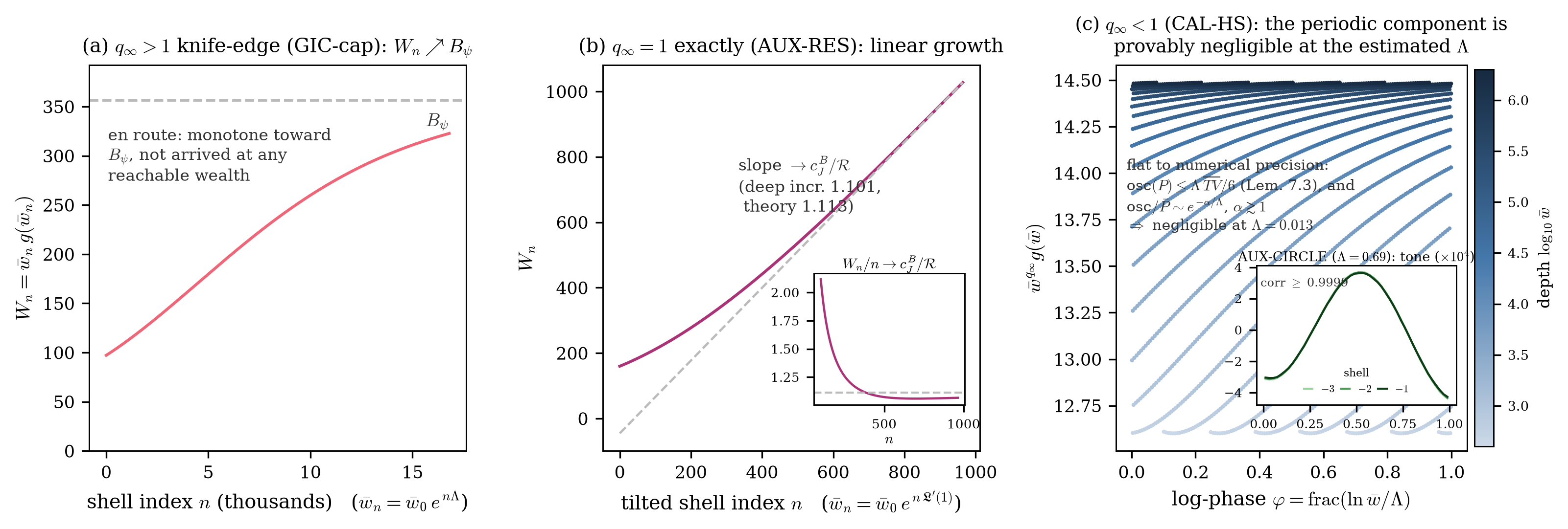
Figure 4:The trichotomy at the boundary. (a) patience ceiling (GIC-CAP): , en route. (b) exactly (AUX-RES): linear growth, . (c) (HS-mean): the periodic component is undetectably small at the estimated calibration’s ; inset — the resolved tone at .
How to read this figure. The three Gordon cases in motion. (a) Convergent case (): the amplitude climbs toward its perpetuity value — a plateau (here honestly en route; see Figure 3a). (b) The knife-edge case ( exactly): no plateau exists; instead value accrues linearly with the rungs of the descent — just as a growing annuity with discount rate equal to growth rate is worth (number of periods) × (per-period flow) — and the slope is the resonance constant (inset: the running average converging to it). This linear accrual is precisely where the extra in the theorem comes from. (c) The case, plotted against the fractional part of log PF wealth: theory says the limit is a periodic function on this axis (a circle, §6), but at HS-mean’s estimated patience the predicted oscillation is — astronomically below any solver’s resolution — so the limit is flat for every practical purpose. The inset shows the one deliberately coarse calibration where the wiggle becomes visible: the circle is real, just irrelevant at realistic patience.
Wrong-exponent detection (Theorem γ-T; PROVEN). Compensate with any other and the boundary behavior degenerates at the exact geometric per-shell rates : ; the true exponent . Two dials govern : the multiplier crosses 1 at , and the forcing () stops fading at — so the only compensation with finite nonzero boundary behavior is . The compactified problem finds the exponent by itself (Figure 5, on HS-mean: trial exponents / drift at measured log-slopes -0.144 / +0.156 against theory -0.15 / +0.15, while stays flat at +0.006; detection rates verified to per shell in the source suite, and reconfirmed on fresh calibrations by the RF2 panel). This doubles as the numerical diagnostic of record: the grid-depth migration of the fitted local exponent toward is a theorem-backed signature, not a stylized fact.
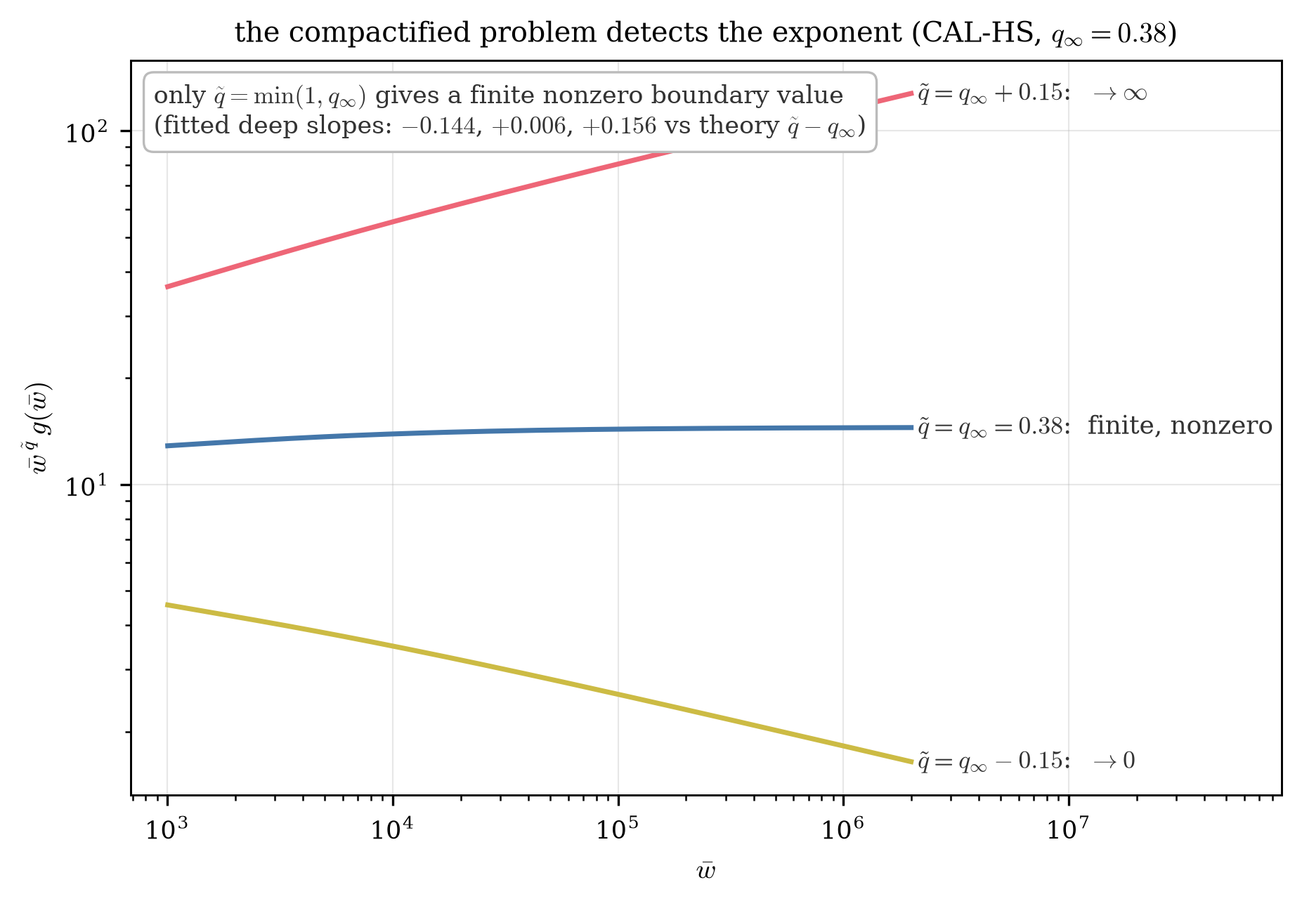
Figure 5:The compactified problem detects the exponent (HS-mean): only gives a finite nonzero boundary value.
How to read this figure. The closest econometric analogy is choosing the right detrending. Multiply the shortfall by a trial power and watch what happens: too small a and the product still dies away (under-compensated); too large and it explodes (over-compensated); exactly right and it levels off. Only levels off — the solved model picks its own exponent, with no fitting involved. This is also §0’s saddle-path selection made visual: wrong exponents put you on explosive or degenerate solution branches.
7. Rigor engine IV: permanent shocks — Theorem III and the human-wealth-revaluation channel¶
(Proof body: alt_proof_compactified.md §7 (γ-B1/γ-B2/γ-B3, Theorem γ-B); Stage-B
foundations imported from stage_B_proof.md §§B1–B3.)
With permanent shocks the exact recursion becomes the master identity
(Watch the typographical neighbors: lowercase is PF total wealth, capital the mean-zero income-revaluation shock — and neither is the compensated gap of §5.) The term is the human-wealth revaluation channel: a permanent shock reprices the entire future income stream — all units of it — so the precautionary forcing is larger than in the transitory-only model. The -weighted one-step relation (B5.2) makes the compactified multiplier , and the identical γ2/γ3 pattern (boundedness via the stopped expectation-unroll Lemma γ-B2, which covers the general bounded- case including the empirically relevant ; key identity ) delivers:
(In words: unroll the expectation of the recursion only up to the random time the state first exits the good region — ‘stopping’ there is legitimate because the displayed identity says the drift is exactly right on average — and boundedness follows without ever tracking an individual path.)
The spine reaches the same constants. §2.6’s -general one-step subtraction (the W3
spike, eq1_backward_psi_spike.md; battery verify_eq1_psi_spike_checks.py) derives the
mode condition — the eigen-equation (26) — and
the amplitude (28) directly from the backward telling, with the discount still
exactly by the (K3) feedback invariance; Theorem III is the rigorous certificate
of that construction at .
Stage-B resonance and are OPEN for this engine (the shell index becomes a
random walk whose occupation control is exactly the original chain’s tilt toolkit); the sharp
results are Theorems B-res, B2, B2-arith of stage_B_proof.md, imported.
(The obstruction, plainly: with permanent shocks the shell index no longer marches down deterministically — each period it moves by a random amount, a random walk with downward drift. Controlling how much time such a walk spends at each level — its ‘occupation’ — is exactly what the exponential-tilting toolkit does for the original Kesten chain; porting that control is the outstanding engineering, not any new economics.)
8. The journey, measured: the economics of the proof¶
§2.4’s unrolling stopped at the log-clock exit — the backward steps end where the descent
reaches the buffer-stock body. Read forward (route α, alt_proof_econlit.md, which prices
the same numbers as a path sum), the gap at PF wealth is the expected present
discounted value of the Kimball precautionary premium (KPP)s the household will still provide along its
buffer-stock journey from down toward the return region around the target
— the precise object behind the phrase “toward the target”, and the destination
this section defines before measuring where along the journey the gap is earned. In BST’s
language
the destination is the individual target (unique under WRIC + FVAC + GIC-Mod
per BST’s buffer-stock-target theorem,
and computable from BST’s implicit equation
) or the pseudo-target
(GIC-Raw).
What the unrolled argument itself consumes is only this: a compact wealth interval
containing the target, on which the descent’s bookkeeping can stop. Concretely (Stage A),
take the PF-wealth levels with — §5.2’s
enlargement constant: above the recursion (8) moves strictly down almost
surely (), from inside the interval PF wealth cannot
exit upward (), the descent from any enters it in
periods, and the target must lie inside (above
PF wealth falls almost surely, contradicting at ). The region is
compact because the transitory shock has bounded support — part of the maintained
income-process assumption (BST,
Assumption assn-shocks;
§1): bounded , with the sandwich , is what makes the
one-step displacement bound — hence the upper edge — finite and computable
from the primitives ( works, read off
(8)). With unbounded transitory shocks the region is not compact — a single large
draw passes any point, no finite exists — and the renewal argument as given needs the
bound; the decay theorem itself still holds via the L4′ moment extension, which replaces the
compact-interval bookkeeping with moment bounds (8.1 How rarely is the tail visited? The dual (Kesten) root, item 3). With permanent
shocks the interval is entered and re-entered rather than absorbing (8.1 How rarely is the tail visited? The dual (Kesten) root,
item 2 quantifies the excursions above it). The journey picture is exactly Carroll’s (1997)
narrative made quantitative. Where along the journey is the gap earned? §2.4 answered in
principle: the head of the journey at , every rung equally at resonance, the
journey’s end at . Figure 6 shows it measured.
The moral for this project: the descent spends ~89% of its lifetime inside any
sensibly-sized grid — the far field is visited too rarely to deserve gridpoints, and what
happens there is exactly what the theory prices. An in-grid representation plus the
theorem’s tail is the whole solution; no ad-hoc external criterion (a grid top, an
extrapolation form, a tolerance) does any work.
Measured on the estimated calibrations (the bookkeeping is the -tilted Wald chain — step , weight per rung — which the figure build verified is the only unroll-consistent accounting at estimated patience): the journey’s-end/boundary share is 89% for HS-mean (, end-dominated), 50% for COL-TOP (, the transition), and 2% for the ceiling GIC-CAP (, head-dominated) — with all three per-rung weights within 1% of 1: estimated patience sits close to the resonance knife-edge, which is the deep reason the historical exponential top-of-grid heuristic was locally harmless even though it is asymptotically wrong (the gap cannot fade faster than the forcing floor — stage-A Lemma 6.1 / stage-B Lemma B-6.1).
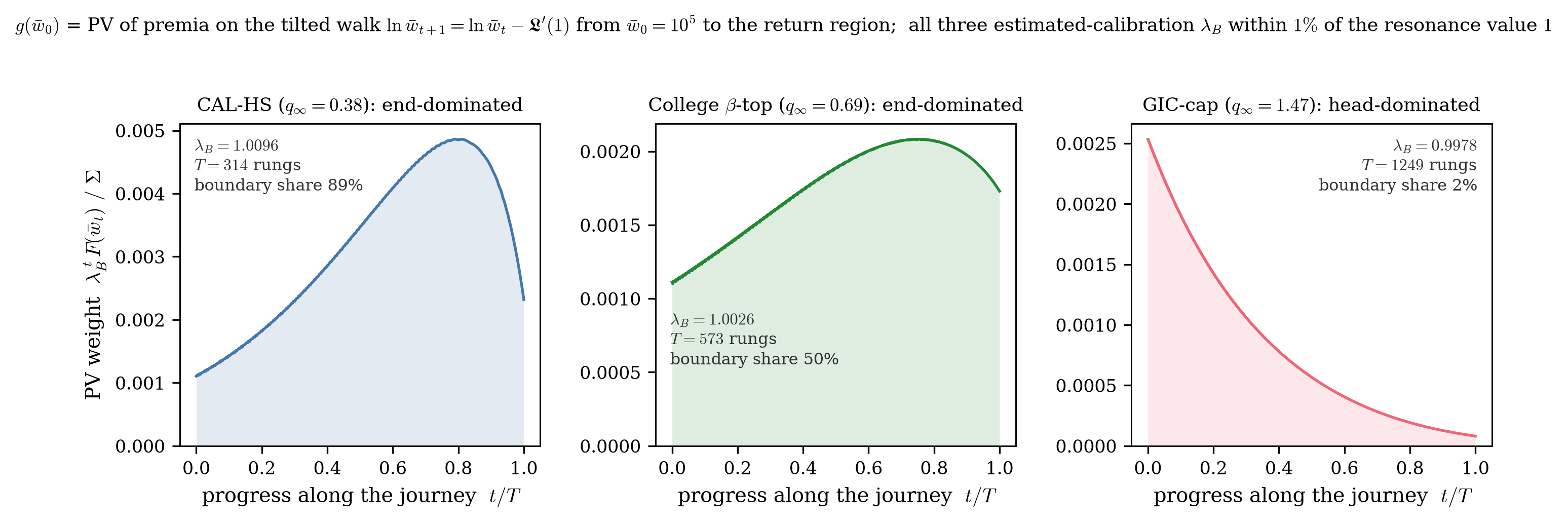
Figure 6:Where the gap is earned along the journey (the three estimated calibrations; ψ²-tilted Wald bookkeeping). Each panel unrolls the pricing recursion rung by rung (one rung = one model period) and plots each rung’s share of the summed rung values; the terminal boundary term is excluded from the normalization and its share is reported separately inside each panel. The moral for this project: the descent spends ~89% of its lifetime inside any sensibly-sized grid — the far field is visited too rarely to deserve gridpoints, and what happens there is exactly what the theory prices. An in-grid representation plus the theorem’s tail is the whole solution; no ad-hoc external criterion (a grid top, an extrapolation form, a tolerance) does any work.
How to read this figure (the “when is the shortfall earned?” decomposition). Recall the buffer-stock reading (§0): the shortfall a wealthy household exhibits today is the present value of the stream of premia it will still provide along its descent toward the target. This figure decomposes that present value by when the premia are provided. The horizontal axis is progress along the descent, rung by rung, rescaled to : 0 = the first rung — today, at PF wealth ; 1 = the last rung providing an adjustment, just above the unroll’s cutoff at — well inside the approach to the target but still above the return region around (8.1 How rarely is the tail visited? The dual (Kesten) root quantifies how rarely the lowest rungs are ever visited). The height is that rung’s share of the summed rung values — the plotted shares sum to one — while the terminal boundary term (the continuation value parked at the cutoff) is excluded from the normalization and reported separately in each panel. Three readings:
HS-mean (): the mass sits at the right. The shortfall of a wealthy high-school-calibration household is almost entirely the discounted shadow of the future — the intense precautionary saving it anticipates doing near the target. Like a growth stock, its value lives in its distant payoffs. (Measured: the terminal boundary term alone carries 89% of the total value.)
Patience ceiling GIC-CAP (): the mass sits at the left. Discounting beats the descent, so value lives in the near adjustments, like a coupon bond’s. (Boundary share: 2%.)
Exact resonance (): flat. Every period of the journey contributes equally — which is exactly why the resonance case picks up the factor: equal contributions.
The punchline for HAFiscal: all three estimated-calibration profiles are close to flat, because the estimated economies sit near the knife-edge (above, the -within-1%-of-1 measurement). That single fact is the deepest reason top-of-grid behavior is delicate at realistic patience: the value of the shortfall is spread almost evenly over the whole journey, so no part of the wealth domain is safely negligible.
8.1 How rarely is the tail visited? The dual (Kesten) root¶
The theorem describes at wealth levels the agent rarely — in one important case never —
holds. This subsection quantifies “rarely”, because the correct quantifier is itself an object
worth knowing: the tail exponent of a Kesten process. (Evidence for every number below:
verify_dualroot_checks.py, ALL PASS, same 7-atom discretization as the figures.)
Economists have met this machine under another name: random growth. Multiply a variable by an i.i.d. factor each period (plus a small additive perturbation); if the factor shrinks on average but sometimes exceeds one, the stationary distribution develops a Pareto upper tail whose exponent solves . This is the mechanism behind Zipf’s law for cities — Gabaix (1999) shows that Gibrat-style proportional random growth of city populations, with a small friction keeping cities from vanishing, produces a power-law size distribution, with the Zipf exponent 1 emerging in the small-friction limit — and the standard account of Pareto tails in wealth and firm size. Gabaix (2009) surveys both the empirical catalog (income and wealth, cities, firms, stock returns, trading volume, executive pay) and the generating theory, including precisely the exponent equation below; Gabaix (2016) is the introduction written for the general economist, arguing these are true quantitative laws — empirically established and theoretically understood. Everything below is that familiar machine, applied to a single household’s normalized perfect-foresight wealth rather than to a cross-section of cities or firms.
Rearranging the master identity (41), normalized perfect-foresight wealth follows
a stochastic recursion with i.i.d. multiplier — the workhorse of the wealth-distribution
literature (Kesten 1973; Goldie 1991; econ packagings Benhabib–Bisin–Zhu 2011, Toda 2014; the
Gouin-Bonenfant–Toda 2023 toolkit’s getZeta computes exactly the object below). The dual
(Kesten) root is the unique solving
which exists precisely when the multiplier (i) contracts on average, , and (ii) occasionally expands, . When it exists, the stationary distribution of has a power tail with exponent : decays essentially like (the upper bound is an elementary Chernoff/supermartingale estimate; the matching lower bound is the Kesten–Goldie theorem, with the usual non-arithmeticity caveat — a discretized technically sits in the lattice case, where Kevei’s 2017 version supplies the log-periodic analogue). Duality made precise: and the theorem’s solve the two members of one Mellin family — the dual equation (45) governs the tail of the wealth distribution; the primal equation (26) governs the approach of the consumption function. §3.2’s obstruction is the case where the dual root fails to exist while the primal always does.
(The caveat, plainly: the clean constant-times-power tail needs the random log-steps of the descent NOT to be all multiples of one common unit. A discretized permanent shock violates that — the ‘lattice’ case — and then the constant is replaced by a bounded periodic wobble in log wealth: the same log-periodic phenomenon as the resonance circle, and equally harmless for the exponent.)
The reachability taxonomy (answering: with random shocks, what can “unreachable” even mean?):
, bounded — literally unreachable. : no expansion, ever; gives an absorbing interval (the return region of §8), so the ergodic support is compact — zero probability beyond a finite point, not merely small. This is the strongest form of §3.2’s contrast: no wealth tail of any kind, yet the gap is exactly a power law.
Permanent shocks, even bounded (the HAFiscal case) — reachable but power-law rare. The 7-atom estimated has at all three calibrations, so : runs of small permanent-income realizations (, so ) shrink the denominator of the normalized ratio and so inflate normalized perfect-foresight wealth without bound — excursions to high normalized PF wealth are produced by bad income luck, not good (the household is income-poor and ratio-rich) — the support is unbounded even though every shock is bounded. “Behaviorally reachable” is then a measure-and-time statement: tail mass , excursions mean-reverting at rate per period.
calibration dual root (Chernoff scale) HS-mean -0.0113 9.19 COL-TOP -0.0039 3.17 GIC-CAP (the patience ceiling) none no stationary from impatience alone Patience fattens the tail ( none) — the familiar patience-to-Pareto mechanism of the wealth-distribution literature, here seen from inside a single agent’s problem.
Unbounded — any level is possible. One large transitory draw passes any point, so there is no finite maximal wealth at all; the ergodic tail then inherits the income tail (Stachurski–Toda 2019). The theorem is indifferent: the L4′ extension covers unbounded .
The patience-ceiling exception. At the GIC-CAP ceiling the mean log-drift is positive: under the reduced i.i.d. dynamics that calibration’s normalized perfect-foresight wealth drifts up forever — impatience alone never pulls it back, and no dual root exists. (As in item 2, the upward drift is a drift of the NORMALIZED ratio, fed by small permanent-income realizations that shrink its denominator — bad income luck, not good.) The cap’s construction pins raw growth impatience to hold — barely () — while the -modified conditions fail ( and ): the raw, log-drift, and expectation-of-ratio conditions are separated by Jensen gaps, and the ceiling calibration sits between raw and modified — an estimated-parameters instance of BST’s condition-lattice distinctions, the case in which GIC-Mod fails while GIC holds, so only the pseudo-target survives. In (2)'s race language the cap’s side effect on the exponent is stark: pinning a hair under 1 kills the descent rate — per quarter, a wealth-ratio half-life of roughly 479 years against a discounting half-life of 34 (§0’s half-life table) — and since the exponent is the ratio discounting/descent, a dead descent rate is precisely what hands the race to discounting: the deterministic ratio is , and only the -tilt of (26) drags the realized root down to 1.47 — supercritical still. The cap and the exponent condition thus pull on the same dial in opposite directions: the cap keeps the solution method safely inside raw growth impatience (§3.1), and does that job; but proximity to the raw-GIC knife-edge is exactly what pushes the exponent past its own boundary — which is why the simplified capstone maintains (its standing assumption, GIC-policy) instead of proximity to the GIC as the discipline on patience. What truncates that calibration’s ergodic normalized PF wealth in the full model (the distribution whose extreme upper quantile fixes the top of the estimation grid) is mortality with replacement — the reset mechanism of the wealth-tail literature (Toda 2014) — and within an expected working life its upward drift moves normalized PF wealth only .
Practical conclusion, sharpened. The asymptotic region — the range on which the gap law’s leading-order form governs and the remainders , are -small — is visited with stationary probability ranging from (HS-mean) down to “only via the mortality-reset tail” (GIC-CAP) — and in the benchmark, never. The theorem’s practical role is therefore exactly as §9 frames it: a boundary condition and extrapolation form for the function, not a description of states to simulate.
9. The computational payoff¶
An in-grid representation plus the theorem’s tail is the whole solution; no ad-hoc external criterion (a grid top, an extrapolation form, a tolerance) does any work.
The boundary value is a boundary condition. Solving on a compactified grid (equivalently, a top-of-grid asymptotic condition) is standard numerical practice; Theorem I upgrades the practice to principle: the exact boundary data at is (), i.e. at the top of the grid — with known in closed form from the calibration.
The extrapolation form of record. The gap extrapolant , , is the asymptotically correct form — the theorem behind the
decay_extrap='powerlaw'flip in the HAFiscal/HARK code (RECONCILED-002; HARK PRfix-aggshock-pf-decay-extrap), replacing the historical exponential heuristic, which decays faster than the forcing floor (stage-A Lemma 6.1 / stage-B Lemma B-6.1) permits as an asymptotic form.The knife-edge window, quantified on HAFiscal’s own numbers. At the estimated calibrations the growth patience factor is close to 1 (), the rescaling is near-additive, and the asymptotic region begins only at astronomically large PF wealth. GIC-CAP makes this concrete: , , — and the compensated gap has covered only 42% of the way to its boundary value at the top of the estimation grid, 91% even at the grid top (Figure 3a). That is why the exponential heuristic was locally harmless on historical grids ( policy effect at the audited window) even though it is asymptotically wrong. The plateau-onset scale quantifies this.
A built-in diagnostic. Theorem γ-T’s detection property is a practical grid test: compensate the measured gap by trial exponents; only stabilizes. The grid-depth migration of fitted exponents toward is the theorem-backed convergence signature for solver validation. The migration’s pace is the purification rate of Figure 1: the fitted exponent’s residual dies like per -fold of grid depth — slowest near resonance.
The computer-science face. In algorithmic terms the sandwich (31)–(32) is a perturbed divide-and-conquer recurrence, and (26) is its Akra–Bazzi critical-exponent equation at ; the trichotomy including the resonance log is the master theorem’s three cases (Akra–Bazzi 1998; Leighton 1996, whose perturbation tolerance — shifts of the recurrence argument up to size at argument — our bounded shifts satisfy with room). That proof is carried out in full in
alt_proof_econcs.md, with hypothesis-match tables against the machine-formalized statements (Isabelle AFPAkra_Bazzi, Eberl 2015/2017; Lean 4 mathlib4Computability/AkraBazzi, with its honest mismatches recorded) and executed interval-arithmetic certificates for , the denominator signs, and / — the certification practice a formalization effort would inherit.The finite-horizon slope, for free. §2.4’s construction makes the truncated sum (21) finite at any finite distance from , so the gap is exactly-order at ANY finite horizon regardless of — the theorem behind the Method of Moderation’s finite-horizon practice: the correct top-of-grid slope is exactly 1 for a finite-horizon solver, and is an infinite-horizon limit statement, not a finite- one.
(The bridge, for economists who have not met divide-and-conquer recurrences: an algorithm that splits a problem into a pieces of a fraction b the size obeys exactly our kind of one-step recursion, level by level; its ‘critical exponent’ equation asks at what power the per-level contributions neither die out nor compound — the same question our root equation asks about backward steps of the journey.)
10. One theorem, four engines — and one telling¶
| engine | document | face | distinctive reach | review |
|---|---|---|---|---|
| backward induction from (the spine, §2) | this document, from eq1_backward_derivation.md | economics / construction | the organizing telling: derives (EQ-1) and unrolls it to every published constant | battery verify_eq1_backward_checks.py: ALL PASS |
| renewal / implicit renewal + tilt | stage_A_proof.md, stage_B_proof.md | classical probability | everything, incl. sharp at (A2/B2/B2-arith), general- resonance (B-res), unbounded (L4′) | R1–4, RB1–4, RC1–4: zero broken |
| journey path-sum (PV of the adjustment stream) | alt_proof_econlit.md | economics | the literature-anchored narrative; general- with no margin condition | RD1/RD2: zero broken |
| perturbed master theorem | alt_proof_econcs.md | computer science | order + constants by induction; formalization anchors + certificates; Stage-B under | RE1/RE2: zero broken |
| compactified boundary fixed point | alt_proof_compactified.md | geometry / computation (this core) | shortest engine; the scalar boundary equation; exponent detection; Cesàro resonance; general- | RF1/RF2: zero broken |
The intellectual division of labor: the spine constructs the theorem backward from the perfect-foresight resumption date and makes every constant visible in one geometric sum; the compactified core proves it the simplest way; the renewal chain proves the most; the path-sum proof tells the same story forward in the economics literature’s language; the master-theorem proof ports it to the community whose tools certify and formalize it.
11. Figures and reproduction¶
All figures are produced by make_final_proof_figures.py (single deterministic run, ~140 s;
12/12 pre-registered checks; log committed as make_final_proof_figures_out.txt); per-figure
provenance and headline numbers are in figures/FIGURES.md, including the calibration table
with source-line citations into the HAFiscal estimation code (HS-mean ;
COL-TOP ; GIC-CAP , ;
resonance auxiliary ) and the honest i.i.d.-reduction caveat (HAFiscal’s
persistent unemployment spells are mapped to an i.i.d. atom at income 0.7 with the
education-specific ergodic unemployment rate). The underlying solvers are the review-pack
EGM libraries (review/R4_egm_lib.py, review/RB4_egm_lib_B.py), run under the program’s
guards (longdouble; tail points quoted only where x/c > 1e-10; large-
calibrations for amplitude exhibits). The theorem-level verification of record is the
pre-registered falsifier suites of the four source documents (all committed with outputs;
31/31, 22/22, 13/15+2-honest-FAILs, and the six refuter packs’ independent batteries).
The spine’s named instrument is verify_eq1_backward_checks.py (pre-registered gates E1–E6
frozen in its header; committed verify_eq1_backward_checks_out.txt), which implements §2’s
backward iteration exactly — pointwise Euler solves against the PF continuation, assembled
in difference form — and checks the one-step law (19), (EQ-1) as an identity
along the iteration, the unrolled amplitude against (27), the exponent, the
resonance slope, and determinism; its -general companion is
verify_eq1_psi_spike_checks.py (§2.6, committed verify_eq1_psi_spike_checks_out.txt).
References¶
Buffer-stock / income-fluctuation foundations. Carroll (1997), QJE 112(1):1–55.
Carroll, Theoretical Foundations of Buffer Stock Saving — cite as NBER WP 10867 (2004) and
forthcoming, Quantitative Economics (no volume/pages exist yet; maintained draft at
llorracc
Precautionary-saving canon. Kimball (1990), Econometrica 58(1):53–73; Kimball (1993), Econometrica 61(3):589–611 (decorative). Pratt (1964), Econometrica 32(1/2):122–136. Arrow (1965/1971), Aspects/Essays in the Theory of Risk-Bearing (lecture volumes). Leland (1968), QJE 82(3):465–473. Sandmo (1970), REStud 37(3):353–360. Drèze–Modigliani (1972), JET 5(3):308–335.
Heavy tails in economics (kinship — the wealth-LEVEL literature; §3.2). Benhabib–Bisin–Zhu (2011), Econometrica 79(1):123–157; (2015), JET 159:489–515. Toda (2014), JET 154:310–348; (2019), JME 104:101–113. Stachurski–Toda (2019), JET 182:1–24 (+ 2020 corrigendum) — the econ-packaged compact-support obstruction. Beare–Toda (2022), Econometrica 90(4):1811–1833. Beare–Seo–Toda (2022), Econometric Theory 38(5):986–1013 (+ corrigendum ET 41(5), 2025). Gouin-Bonenfant–Toda (2023), Quantitative Economics 14(1):201–233 (+ the Pareto-extrapolation toolkit).
Power laws in the random-growth canon (§0 and 8.1 How rarely is the tail visited? The dual (Kesten) root). Gabaix (1999), “Zipf’s Law for Cities: An Explanation,” QJE 114(3):739–767 — shows that proportional random growth (Gibrat’s law) with a small friction preventing collapse to zero generates a power-law city-size distribution, and that the Zipf exponent of 1 emerges in the small-friction limit; the template for “random growth ⟹ Pareto tail.” Gabaix (2009), “Power Laws in Economics and Finance,” Annu. Rev. Econ. 1:255–294 — the survey of the empirical power laws (income and wealth, cities, firms, stock returns, trading volume, executive pay) and of the random-growth/Kesten theory that generates them, including the exponent equation used in 8.1 How rarely is the tail visited? The dual (Kesten) root. Gabaix (2016), “Power Laws in Economics: An Introduction,” J. Econ. Perspect. 30(1):185–206 — the economist-facing introduction arguing that these are true quantitative laws, both empirically established and theoretically understood.
Probability engines (used by the original chain). Kesten (1973), Acta Math. 131:207–248. Goldie (1991), Ann. Appl. Probab. 1(1):126–166. Athreya–McDonald–Ney (1978), Ann. Probab. 6(5):788–797. Grincevičius (1975); Grey (1994), AAP 4(1):169–183; Vervaat (1979); Kevei (2017), J. Appl. Probab. 54(3):732–749 (+ 2016 ECP note). Buraczewski–Damek–Mikosch (2016), Springer (Thms 2.4.4/2.4.7). Jelenković–Olvera-Cravioto (2012), AAP 44(2):528–561.
Divide-and-conquer / formalization (the CS face; §9.5). Akra–Bazzi (1998), Comput. Optim. Appl. 10(2):195–210. Leighton (1996), MIT ms. Eberl (2017), J. Automated Reasoning 58(4):483–508
Isabelle AFP
Akra_Bazzi(2015). mathlib4Computability/AkraBazzi(Dupuis, 2023). Drmota–Szpankowski (2013), J. ACM 60(3): Art. 16. Flajolet–Golin (1994), Acta Informatica 31(7):673–696. Karp (1994), J. ACM 41(6):1136–1150. Roura (2001), J. ACM 48(2):170–205.
Compactification ancestry. Dumortier–Llibre–Artés (2006), Qualitative Theory of Planar Differential Systems, Springer, ch. 5.