Solution Methods for Microeconomic
Dynamic Stochastic Optimization Problems
2026-03-11
Christopher D. Carroll1
Note: The GitHub repo SolvingMicroDSOPsassociated with this document contains python code thatproduces all results, from scratch, except for the last section on indirect inference. The numerical results havebeen confirmed by showing that the answers that the raw python produces correspond to the answersproduced by tools available in the Econ-ARKtoolkit, more specifically those in the HARKwhichhas full documentation. The MSM results at the end have have been superseded by tools in theEstimatingMicroDSOPs repo.
Abstract These notes describe tools for solving microeconomic dynamic stochastic optimization problems,and show how to use those tools for efficiently estimating a standard life cycle consumption/savingmodel using microeconomic data. No attempt is made at a systematic overview of the many possibletechnical choices; instead, I present a specific set of methods that have proven useful in my own work(and explain why other popular methods, such as value function iteration, are a bad idea).Paired with these notes is Python code that solves the problems described in the text.
(Contains LaTeX code for this document and software producing figures and results)
1Carroll: Department of Economics, Johns Hopkins University, Baltimore, MD, ccarroll@jhu.eduThe notes were originally written for my Advanced Topics in Macroeconomic Theoryclass at Johns Hopkins University; instructors elsewhere are welcome to use them forteaching purposes. Relative to earlier drafts, this version incorporates several improvementsrelated to new results in the paper “Theoretical Foundations of Buffer Stock Saving”(especially tools for approximating the consumption and value functions). Like the last majordraft, it also builds on material in “The Method of Endogenous Gridpoints for SolvingDynamic Stochastic Optimization Problems” published in Economics Letters, available athttp://www.econ2.jhu.edu/people/ccarroll/EndogenousArchive.zip, and by including samplecode for a method of simulated moments estimation of the life cycle model a la ? and Cagetti (?).Background derivations, notation, and related subjects are treated in my class notes for first year macro,available at http://www.econ2.jhu.edu/people/ccarroll/public/lecturenotes/consumption. Iam grateful to several generations of graduate students in helping me to refine these notes, to MarcChan for help in updating the text and software to be consistent with ?, to Kiichi Tokuoka for draftingthe section on structural estimation, to Damiano Sandri for exceptionally insightful help in revising andupdating the method of simulated moments estimation section, and to Weifeng Wu and Metin Uyanikfor revising to be consistent with the ‘method of moderation’ and other improvements. All errors aremy own. This document can be cited as ? in the references.
1 Introduction
These notes provide a gentle-as-possible introduction to a particular set of
solution tools for the canonical consumption-saving/portfolio allocation problem
for a consumer facing uninsurable idiosyncratic risk to nonfinancial income
(e.g., labor or transfer income), first without and then with optimal portfolio
choice,1
with detailed intuitive discussion of various mathematical and computational techniques that,
together, accelerate the solution by many orders of magnitude. The problem is solved with and
without liquidity constraints, and the infinite horizon solution is the limit of the finite horizon
solution. After the basic consumption/saving problem with a deterministic interest rate is
described and solved, an extension with portfolio choice between a riskless and a risky asset is
also solved. Finally, a simple example shows how to use these methods (via the statistical
‘method of simulated moments’ (MSM for short)) to estimate structural parameters
like the coefficient of relative risk aversion (a la Gourinchas and Parker (?) and
Cagetti (?)).
2 The Problem
The usual analysis of dynamic stochastic programming problems packs a great many events
(intertemporal choice, stochastic shocks, intertemporal returns, income growth, the taking of
expectations, time discounting, and more) into a complex decision in which the agent
makes an optimal choice simultaneously taking all these elements into account.
For the dissection here, we will be careful to break down everything that happens
into distinct operations so that each element can be scrutinized and understood in
isolation.
We are interested in the behavior of a consumer who begins period
with a
certain amount of ‘capital’
(1)
which immediately earns a return factor .
Simultaneously, the consumer receives noncapital income
, which is the product
of ‘permanent income’
and a transitory shock :
(2)
whose expectation is 1 (that is, before realization of the transitory shock, the consumer’s
expectation is that actual income will on average be equal to permanent income
).
The combination of the capital return and income defines the consumer’s ‘market resources’
(sometimes called ‘cash-on-hand,’ following ?):
(3)
available to be spent on consumption
for a consumer subject to a liquidity constraint that requires
(though we are not imposing such a constraint yet—see subsection 6.8). Finally we define
(4)
mnemonically as ‘assets-after-all-actions-are-accomplished.’
The consumer’s goal is to maximize discounted utility from consumption over the rest of a lifetime
ending at date :
(5)
(6)
Income evolves according to:
(7)
(8)
Equation (8) indicates that we are allowing for a predictable average profile of income growth over
the lifetime
(to capture typical career wage paths, pension arrangements,
etc).2
Finally, the utility function is of the Constant Relative Risk Aversion (CRRA) form,
.
It is well known that this problem can be rewritten in recursive (Bellman) form:
(9)
(10)
subject to the Dynamic Budget Constraint (DBC) defined by equation (3), and to the
dynamic process for income defined in (8) and to a transition equation that defines next
period’s initial capital as this period’s end-of-period assets:
(11)
3 Normalization
The single most powerful method for speeding the solution of such models is to redefine the
problem in a way that reduces the number of state variables (if at all possible). In the
consumption context, the obvious idea is to see whether the problem can be rewritten in
terms of the ratio of various variables to permanent noncapital (‘labor’) income
(henceforth for brevity, ‘permanent income.’)
In the last period of life ,
there is no future value,
(boldface
denotes the value function in levels; the nonbold normalized counterpart
is
defined below), so the optimal plan is to consume everything:
(12)
Now define nonbold variables as the bold variable divided by the
level of permanent income in the same period, so that, for example,
; and define
.3
For our CRRA utility function, ,
so (12) can be rewritten as
(13)
Because we are dividing
level variables by ,
a normalized return factor emerges:
(14)
(We treat
as time-invariant and drop the period subscript that appeared in (3).)
Now define a new optimization problem:
(15)
(16)
Then it is easy to see that for , we
can write boldface (nonnormalized)
as a function of
(normalized value) and permanent income:
(17)
and so on back to all earlier periods (by backward induction: if the factorization holds at
, substituting into the
Bellman equation at
and using the homogeneity of CRRA utility yields the same factorization at
).
Hence, if we solve the problem (16) which has only a single state variable
, we can
obtain the levels of the value function from (17), and of consumption and all other variables
from the corresponding permanent-income-normalized solution objects by multiplying each by
,
e.g.
We have thus reduced the problem from two continuous state variables to one (and thereby enormously
simplified its solution).4
For future reference it will be useful to write (16) in the traditional way, by substituting
and
into
:
(18)
4 Notation
4.1 Periods, ,
The problem so far assumes that the agent has only one decision. But agents often have multiple
choices per period—for example, a consumption decision, a labor supply choice, and a choice of what
proportion
of capital
to invest in a risky vehicle. We identify each type in two ways: by a short-name (a textual
name, given when the stage is first introduced) and by a control-name (the stage’s control
variable, if any). For example, a labor supply might have short-name labor and control-name
; a consumption
has control-name .
A stage list that constitutes a period may therefore be written by short-name,
e.g. , or by
control-name, e.g. .
A modeler might want to explore whether the order in which the are solved makes any
difference, either to the substantive results or to aspects of the computational solution like
speed and accuracy; with this scheme they do so merely by changing the order in which the
stages are listed in the specification of the period.
If, as in section 2, we hard-wire into the solution code for each an assumption that its
successor will be something in particular (say, the consumption assumes that the portfolio
choice is next), then if we want to change the order of the (say, labor supply after
consumption, followed by portfolio choice), we will need to re-hard-wire each of the stages to
know new things about its new successor (for example, the specifics of the distribution of the
rate of return on the risky asset must be known by whatever precedes the portfolio choice
).
The cardinal insight of ? is that everything that matters for the solution to the current
problem is encoded in a ‘continuation-value function.’
Using that insight, we describe here a framework for isolating the problems within a period
from each other, and the period from its successors or predecessors in any other period. The
advantage of this isolation is that each problem becomes a self-contained module: Its internal
logic—the computation it performs on value functions—is defined independently of where it
sits in the sequence of .
Modularity is valuable because it makes exploring such alternative model
structures cheap. Using control-name indexing (e.g., the consumption by
), after considering
the -order ,
the modeler can reorder the to consider, say, the order
without rewriting any of the code that solves each individual
.5
What must change are the transitions—the mappings that connect the end of one to the
beginning of the next—which must be rewired to reflect the new ordering and its implied
information structure. The -level code itself remains untouched.
4.2
The key is to distinguish, within each ’s Bellman problem, three viewpoints or ‘’ (we use that
word to empasize that the does not do anything: It is merely a collection of mathematical and
computational functions and objects).
: Incoming state variables (e.g., )
are known, but any shocks associated with the have not been realized and
decision(s) have not yet been made
: The agent solves the decision problem for the period
: After all decisions have been made, their consequences are measured by evaluation
of the continuing-value function at the values of the ‘outgoing’ state variables
(sometimes called ‘post-state’ variables)
This framework is deliberately silent about when shocks (if any) occur within a . Shocks may be
realized between the and , or between the and —the choice is part of the ’s specification,
not a framework-level constraint. In a consumption problem, the usual assumption is that
income shocks have been realized before the spending decision is made, so that the consumer
knows their resources when they decide how much to spend; here, shocks fall between and
().
But in a portfolio choice problem, the portfolio share decision must be
made before the return shock is realized; there, shocks fall between and
().
The structure accommodates both patterns: the -to- relationship encodes
pre-decision uncertainty, while the -to- relationship encodes post-decision
uncertainty. A with no shocks at all (such as cons-noshocks or disc) simply sets
or
with
no intervening expectation.
Table 1: within the cons-with-shocks
Indicator
State
value functions
Explanation
value at entry to
(s)
value of -decision
value at exit
This cons-with-shocks corresponds to the consumption problem defined above.
The table illustrates notation we can use when analyzing the problem from
a context ‘inside’ a particular stage of a specific period. We require that no
variable can have more than one meaning or interpretation inside a period, and
we prohibit any reference to values of any variables or functions or other model
objects from outside the stage (or period). This is why we use different letters,
and
, to represent liquid
resources before and after the consumption decision, even if ultimately this period’s continuation value of
will transmute into the
next period’s initial .
(Both
and are
“k-type” variables—investable capital before returns are realized; the distinction from “m-type”
variables like ,
which represent spendable resources after returns, is formalized below.)
In contrast, items like value functions
or expectations operators
have different meanings at different perches; we capture this using a subscript like
.
The fact that all functions in a perch depend on the same state variables (shown
in the second column) allows us to write those functions without specifying their
arguments.
4.3 Builders and Connectors
Modularity requires that objects inside a period have no direct access to
objects from any other period. This means that we must endow a or a
period, at the time of its creation, with its end-of–or-period value function
.
For example, in a model in which every period contains only the single-stage consumption
problem above, the continuation value function for the last (and only) stage at will need to be
’connected’ to the arrival value function in (+1), which of necessity requires us to use
-related notation. Concretely, if we designate the end-of-period value function as
(which
is defined as the continuation value function from the last in the period), we use the notation
(19)
to describe what the builder does when constructing the predecessor to period
. The use
of the ‘’
signals creation: the left-hand side is brought into existence by the builder.
Expectation operators across .
The subscript on an expectation operator
indicates the
information set at that :
conditions on the state but not on any shocks realized between and . For adjacent at a period
boundary—
( of period )
and ( of
period )—the
information sets are identical, so the two operators are mathematically
interchangeable; the notational distinction reflects viewpoint (looking backward from
’s exit versus
forward from ’s
entry).
Tying two adjacent or periods together also requires that we define a ,
, which
specifies the relationship between the continuation-perch state variable(s) of the predecessor to
the arrival-perch state variable(s) of the successor. Again concretely, for two successive periods
each of which contains only a single consumption like the one described above, the would
look like:
(20)
State-variable types.
Every state variable in the framework belongs to exactly one of two types:
k-type (capital): investable assets before returns and income are realized.
The defining characteristic is that a k-type variable must pass through a
returns-and-shocks process before it becomes spendable. Examples:
(beginning-of-period capital) and
(end-of-period assets after consumption, awaiting next period’s returns).
m-type (market resources): spendable resources after returns and income shocks
have been realized—what ? calls “cash-on-hand.” The defining characteristic is that
an m-type variable is immediately available for spending or allocation decisions.
Examples:
(market resources at the ) and
(post-shock market resources within a period).
Well-typed connectors. A is a pure rename: it asserts that two variables from adjacent or
periods are different names for the same economic object. A is well-typed if and only if the
two variables it connects share the same type. Thus:
is well-typed: both are k-type.
is well-typed: both are m-type.
would be illegal:
is m-type and
is k-type. Market resources and investable capital are not merely different
names for the same quantity—converting between them requires a substantive
transformation (the realization of returns and income). Attempting such a
connector is a modeling error: it would silently skip the returns process, treating
post-return resources as if they were pre-return capital.
The type constraint prevents a common class of modeling errors in which a modeler
inadvertently connects a post-return variable to a pre-return slot (or vice versa), producing
economically nonsensical dynamics. By requiring type agreement, the framework ensures that
every transition between k-type and m-type passes through an explicit returns-and-shocks
.
Annotating stage tables with types.
When reading the tables in this document and in section 9, the arrival and continuation
state types can be read off directly:
disc: arrival and continuation inherit the type of the predecessor’s exit state
(passthrough).
A within-period between two must respect the same type constraint: the predecessor ’s
continuation type must match the successor ’s arrival type.
Namespace uniqueness and the decoration.
A strict rule of the framework is that each variable name refers to exactly one valuewithin a given period. This namespace uniqueness constraint ensures that the mapping
between mathematical symbols and computational variables (e.g., Python names) is
well-defined: if a symbol appears in an equation, there is no ambiguity about which quantity it
denotes.
The constraint has a practical consequence when multiple within the same period
produce variables of the same type. For example, in the portable–consnoshocks
period (section 9.2.5.0), the portable produces post-shock market resources, and the
cons-noshocks receives market resources as its state. Both quantities are m-type, but
they arise at different points in the period and generally take different values. To
preserve namespace uniqueness, the earlier occurrence receives a decoration: we write
for the portable ’s output
and for the cons-noshocks
’s input. The within-period
then renames one to the other.
More generally, when a ’s continuation state has the same type as another ’s arrival state
within the same period, the later or secondary occurrence may receive a decoration
(,
, etc.)
to maintain uniqueness. The decoration signals that the variable is of the same economic type
as its undecorated counterpart but occupies a distinct position in the period’s computation.
This convention makes it straightforward to translate the mathematical notation into code:
each decorated symbol maps to a unique Python variable name (e.g., mNrmCheck for
, mNrm
for ),
and no variable is overwritten or reused within a single period’s scope.
4.4 The Pile: Definition and Construction
4.4.1 Formal Definition
The pile
is an ordered sequence of solved periods interleaved with the that join them. Formally, a pile
with
periods is:
(21)
where each
is a solved period (containing its stage list, value functions, and policy functions) and each
is a
between-period satisfying the type constraint from section 4.3: the predecessor’s exit state
and the successor’s entry state must share the same type (k-type or m-type).
The pile is well-formed if and only if every adjacent
triple
satisfies:
Type consistency. The continuation-state type of ’s
last matches the arrival-state type of ’s
first , and the is a valid rename between them.
Value-function compatibility. The and builder together produce a
continuation value function for
from the arrival value function of .
4.4.2 The Consumption-Only Pile
For the consumption-only problem of sections 2–3, each period contains the stage list
(or, in the single-
formulation, just ).
The between-period is
(both k-type). A three-period consumption-only pile is therefore:
4.4.3 Homogeneous and Heterogeneous Piles
A pile is homogeneous if every period has the same stage list, the same parameter values, and
the same between-period . The infinite-horizon consumption problem (section 7) converges to a
homogeneous pile: every period is identical, and the converged solution is a fixed point of the backward
builder .
A pile is heterogeneous if periods differ in their stage lists, parameter values, or . A life cycle
model is typically heterogeneous: mortality risk, income profiles, and available choices (e.g.,
whether portfolio optimization is active) may vary by age. For example, a life cycle model might
use
for working-age periods (with active portfolio choice) and
for
retirement periods (no portfolio choice).
4.4.4 Backward Construction
We call the structure in which accumulating periods are stored the pile
.
Once backward induction is complete, the pile holds the full definition of the solved
problem.
The process of building the pile is straightforward. We start from the terminal period (section 3:
, consume everything),
so initially . We denote
the backward builder as .
Applying to
the existing
creates a new and then the new period’s solution, yielding
. Each subsequent
application of
prepends one more
pair, growing the pile from right to left. Section 6 details the construction of
; with
multiple or control variables the structure generalizes as in section 9.
5 The Usual Theory, and a Bit More Notation
For reference and to illustrate our new notation, we will now derive the Euler
equation and other standard results for the problem described above. Since
we can write value as of the end of the consumption stage as a function of
:
(22)
Derivative notation convention.
Throughout this document, a
superscript
on a function means its derivative with respect to the relevant state variable at that perch:
,
.
So, the first order condition for (18) with respect to
6
is
(23)
which illustrates the derivative convention
(e.g. is the derivative
of with respect
to its argument).7
For functions of more than one argument, we append the variable name:
denotes the partial
derivative of
with respect to .
we can substitute the LHS of (24) for the RHS of (23) to get
(25)
(26)
and rolling forward one period,
(27)
so that substituting the LHS in equation (23) finally gives us the Euler equation for
consumption:
(28)
(29)
The derivation above used period-qualified subscripts (e.g.,
,
)
because the Euler equation relates objects across periods. We can now restate the
problem (18) using the simpler within- notation, which drops the period qualifier:
(30)
whose first order condition with respect to
is
(31)
which is mathematically equivalent to the usual Euler equation for consumption.
We will revert to this formulation when we reach subsection 6.9.
6 Solving the Next-to-Last Period
This section examines the second-to-last period in detail, illustrating a number of powerful
techniques for speeding and improving its solution; in doing so it illustrates how the pile
(subsection 4.4) is
built backward. We set
here to reduce clutter.
6.1 A Direct Expression for
If , the
second-to-last-period decision-perch problem is
(32)
Using (0) ;
(1) ; (2) the
definition of ;
and (3) the definition of the expectations operator,
(33)
where is the cumulative
distribution function for ,
this maximization problem implicitly defines a ‘period-and–local function’
that yields optimal consumption
in period for any specific
numerical level of resources like .
The explicit statement of the problem is
(34)
But because there is no general analytical solution, for any given
we must use numerical
tools to find the
that maximizes the expression. This is excruciatingly slow: for every candidate
, a definite
integral over
must be calculated numerically, and optimization is itself a costly operation, so the
combination of the two is a double-whammy for slowdown.
6.2 Discretizing the Distribution
Our first speedup trick is therefore to construct a discrete approximation to the lognormal distribution
that can be used in place of numerical integration. That is, we want to approximate the expectation over
of a function
by calculating its
value at set of points
, each of which has an
associated probability weight :
(because adding
weighted values to each other is enormously faster than general-purpose numerical
integration).
Such a procedure is called a ‘quadrature’ method of integration; ? survey
a number of options, but for our purposes we choose the one which is easiest to
understand: An ‘equiprobable’ approximation (that is, one where each of the values of
has an equal
probability, equal to ).
We calculate such an -point
approximation as follows.
Define a set of points from
to on the
interval as the elements of the set
.8
Call the inverse of the
distribution , and define the
points . Then the conditional
mean of in each of the
intervals numbered 1 to
is:
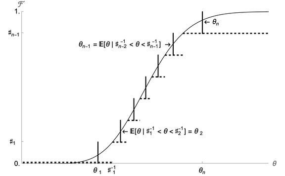
(35)
and when the integral is evaluated numerically for each
the result is a set of values
of that correspond to the
mean value in each of the
intervals.
The method is illustrated in Figure 2. The solid continuous curve represents the “true” CDF
for a lognormal
distribution such that ,
. The short vertical line segments
represent the equiprobable
values of which are used to
approximate this distribution.9
Figure 1: Equiprobable Discrete Approximation to Lognormal Distribution
Figure 2: Equiprobable Discrete Approximation to Lognormal Distribution
The following notebook snippet constructs these points.
(36)
We now substitute our approximation (37) for
in (32) which is
simply the sum of
numbers and is therefore easy to calculate (compared to the full-fledged numerical integration
(33)
that it replaces).
(37)
6.3 The Approximate Consumption and Value Functions
Given any particular value of ,
a numerical maximization tool can now find the
that
solves (32) in a reasonable amount of time.
The notebook responsible for computing an estimated consumption function begins in “Solving
the Model by Value Function Maximization,” where a vector of possible values of market resources
is created. In these
notes we use for
such a vector (e.g.
the first entry,
the last). For illustration we take the grid to be the first five nonnegative integers,
.
6.4 An Interpolated Consumption Function
This is accomplished in “An Interpolated Consumption Function,” which generates an interpolating function
that we designate .
Figures 3 and 4 show plots of the constructed
and
. While the
function looks very
smooth, the fact that the
function is a set of line segments is very evident. This figure provides the beginning of the
intuition for why trying to approximate the value function directly is a bad idea (in this
context).10
Figure 3:
(solid) versus
(dashed)
Figure 4:
(solid) versus
(dashed)
6.5 Interpolating Expectations
Piecewise linear ‘spline’ interpolation as described above works well for generating a
good approximation to the true optimal consumption function. However, there is
a clear inefficiency in the program: Since it uses equation (32), for every value of
the program must calculate the utility consequences of various possible choices of
(and
therefore )
as it searches for the best choice.
For any given index
in , as it searches for the
corresponding optimal , the
algorithm will end up calculating
for many values close to the
optimal . Indeed, even when
searching for the optimal
for a different
(say for
) the search process
might compute
for an close to the
correct optimal
for .
But if that difficult computation does not correspond to the exact solution to the
problem, it is discarded.
The notebook section “Interpolating Expectations,” now interpolates
the expected value of ending the period with a given amount of
assets.11
Figure 5 compares the true value function to the approximation produced by following the
interpolation procedure; the approximated and exact functions are of course identical at the
gridpoints of
and they appear reasonably close except in the region below
.
Figure 5: End-Of-Period Value
(solid) versus
(dashed)
Figure 6:
(solid) versus
(dashed)
Nevertheless, the consumption rule obtained when the approximating
is used
instead of
is surprisingly bad, as shown in figure 6. For example, when
goes from 2 to 3,
goes from about 1 to
about 2, yet when
goes from 3 to 4,
goes from about 2 to about 2.05. The function fails even to be concave, which is distressing
because Carroll and Kimball (?) prove that the correct consumption function is strictly
concave in a wide class of problems that includes this one.
6.6 Value Function versus First Order Condition
Loosely speaking, our difficulty reflects the fact that the consumption choice is
governed by the marginal value function, not by the level of the value function
(which is the object that we approximated). To understand this point, recall
that a quadratic utility function exhibits risk aversion because with a stochastic
,
(38)
(where
is the ‘bliss point’ which is assumed always to exceed feasible
).
However, unlike the CRRA utility function, with quadratic utility the consumption/saving
behavior of consumers is unaffected by risk since behavior is determined by the first order
condition, which depends on marginal utility, and when utility is quadratic, marginal utility is
unaffected by risk:
(39)
Intuitively, if one’s goal is to accurately capture choices that are governed by marginal
value, numerical techniques that approximate the marginal value function will yield a more
accurate approximation to optimal behavior than techniques that approximate the level of the
value function.
The first order condition of the maximization problem in period
is:
(40)
(41)
Figure 7:
versus
The downward-sloping curve in Figure 7 shows the value of
for our baseline
parameter values for
(the horizontal axis). The solid upward-sloping curve shows the value of the RHS of (41) as a function of
under the assumption
that . Optimal
consumption given is the
at which the two curves
intersect—just below . The
dashed curve shows the same for ;
its intersection with
is slightly below ,
so increasing
from 3 to 4 raises optimal consumption by about 0.5.
Now consider the derivative of .
Because the function is piecewise linear, its derivative
is a
step function: constant between adjacent gridpoints, with jumps at each gridpoint.
The solid-line step function in Figure 7 depicts the actual value of
. When we attempt to
find optimal values of
given using
, the numerical optimization
routine will return the
for which . Thus, for
the program will return
the value of for which
the downward-sloping
curve intersects with the ;
as the diagram shows, this value is exactly equal to 2. Similarly, if we ask the routine to find the
optimal for
, it finds the point
of intersection of
with ;
and as the diagram shows, this intersection is only slightly above 2. Hence, this figure
illustrates why the numerical consumption function plotted earlier returned values very close
to for
both
and .
We would obviously obtain much better estimates of the point of intersection between
and
if our
estimate of
were not a step function. In fact, we already know how to construct linear interpolations to
functions, so the obvious next step is to construct a linear interpolating approximation to
the expected marginal value of end-of-period assets function at the points in
:
(42)
yielding (the vector of expected
end-of-period- marginal values
of assets corresponding to ),
and construct
as the linear interpolating function that fits this set of points.
Figure 8:
versus
The results are shown in Figure 8. The linear interpolating approximation looks roughly as
good (or bad) for the marginal value function as it was for the level of the value function.
However, Figure 9 shows that the new consumption function (long dashes) is a
considerably better approximation of the true consumption function (solid) than was the
consumption function obtained by approximating the level of the value function (short
dashes).
Figure 9:
(solid) Versus Two Methods for Constructing
6.7 Transformation
Even the new-and-improved consumption function diverges notably from the true solution, especially at
lower values of .
That is because the linear interpolation does an increasingly poor job of capturing the nonlinearity of
at lower and
lower levels of .
This is where we unveil our next trick. To understand the logic, start by considering the case
where
and there is no uncertainty (that is, we know for sure that income next period will be
).
The final Euler equation (recall that we are still assuming that
) is
then:
(43)
In the case we are now considering with no uncertainty and no liquidity constraints, the optimizing
consumer does not care whether a unit of income is scheduled to be received in the future period
or the
current period ;
there is perfect certainty that the income will be received, so the consumer treats its PDV as
equivalent to a unit of current wealth. Total resources available at the point when the
consumption decision is made is therefore comprised of two types: current market resources
and ‘human wealth’ (the
PDV of future income) of
(because it is the value of human wealth as of the end of the period, there is only one more
period of income of 1 left).
(44)
Of course, this is a highly nonlinear function. However, if we raise both sides of (44) to the
power
the result is a linear function:
(45)
This is a specific example of a general phenomenon: A theoretical literature discussed in ?
establishes that under perfect certainty, if the period-by-period marginal utility function is of the form
, the marginal value
function will be of the form
for some constants .
This means that if we were solving the perfect foresight problem numerically, we could always
calculate a numerically exact (because linear) interpolation.
The key insight is that much of the nonlinearity in
comes from raising to the
power . By inverting that
operation (raising to ),
we can ‘unwind’ it, and the remaining nonlinearity is much smaller.
Specifically, applying the foregoing insights to the end-of-period value function
, we
can define an ‘inverse marginal value’ function
(46)
which would be linear in the perfect foresight
case.12
We then construct a piecewise-linear interpolating approximation to the
function,
, and for any
that falls in
the range
we obtain our approximation of marginal value from:
(47)
The most interesting thing about all of this, though, is that the
function has another interpretation. Recall our point in (31) that
. Since with
CRRA utility ,
this can be rewritten and inverted
(48)
This gives a concrete
interpretation: for any ending ,
it reveals how much the agent must have consumed to (optimally) reach that
. We
will therefore henceforth refer to it as the ‘consumed function:’
(49)
Thus, for example, for period our
procedure is to calculate the vector of
points on the consumed function:
(50)
with the idea that we will construct an approximation of the consumed function
as the interpolating
function connecting these
points.
6.8 The Natural Borrowing Constraint and the
Lower
Bound
This is the appropriate moment to ask an awkward question: How
should an interpolated, approximated ‘consumed’ function like
be extrapolated to return an estimated ‘consumed’ amount when evaluated at an
outside the range
spanned by ?
For most canned piecewise-linear interpolation tools like scipy.interpolate, when the
‘interpolating’ function is evaluated at a point outside the provided range, the algorithm
extrapolates under the assumption that the slope of the function remains constant beyond its
measured boundaries (that is, the slope is assumed to be equal to the slope of nearest
piecewise segment within the interpolated range); for example, if the bottommost gridpoint is
and the corresponding
consumed level is
we could calculate the ‘marginal propensity to have consumed’
and construct the approximation as the linear extrapolation below
from:
(51)
To see that this will lead us into difficulties, consider what happens to the true (not approximated)
as
approaches a quantity we will call the ‘natural borrowing constraint’:
. From
(42)
we have
(52)
But since , exactly at
the first term in the summation
would be which is infinity.
The reason is simple: is the
PDV, as of , of the minimumpossible realization of income in
().
Thus, if the consumer borrows an amount greater than or equal to
(that is, if the
consumer ends
with )
and then draws the worst possible income shock in period
, they will have to
consume zero in period ,
which yields
utility and
marginal utility.
As ? first noticed, this means that the consumer faces a ‘self-imposed’
(or, as above, ‘natural’) borrowing constraint (which springs from the
precautionary motive): They will never borrow an amount greater than or equal to
(that is, assets will never
reach the lower bound of ).
The constraint is ‘self-imposed’ in the precise sense that if the utility function were different
(say, Constant Absolute Risk Aversion), the consumer might be willing to borrow more than
because a choice of zero or negative consumption in period
would yield some finite
amount of utility.13
This self-imposed constraint cannot be captured well when the
function is approximated by a piecewise linear function like
,
because it is impossible for the linear extrapolation below
to correctly
predict
So, the marginal value of saving approaches infinity as
. But this
implies that ;
that is, as
approaches its ‘natural borrowing constraint’ minimum possible value, the corresponding amount of
worst-case
must approach its lower bound: zero.
The upshot is a realization that all we need to do to address these problems is to prepend each
of the and
from (50)
with an extra point so that the first element in the mapping that produces our interpolation
function is .
This is done in section “The Self-Imposed ‘Natural’ Borrowing Constraint and the
Lower
Bound” of the notebook.
Figure 10: True
vs its approximation
Figure 10 shows the result. The solid line calculates the exact numerical value of the consumed
function
while the dashed line is the linear interpolating approximation
This
figure illustrates the value of the transformation: The true function is close to linear, and so the
linear approximation is almost indistinguishable from the true function except at the very lowest
values of .
Figure 11 similarly shows that when we generate
using our
augmented
(dashed line) we obtain a much closer approximation to the true marginal value function
(solid
line) than we obtained in the previous exercise which did not do the transformation
(Figure 8).
Figure 11: True
vs.
Constructed Using
6.9 The Method of Endogenous Gridpoints (‘EGM’)
The solution procedure above for finding
still requires us, for each point in ,
to use a numerical rootfinding algorithm to search for the value of
that
solves .
Though sections 6.7 and 6.8 developed a highly efficient and accurate procedure to calculate
, those
approximations do nothing to eliminate the need for using a rootfinding operation for calculating, for
an arbitrary ,
the optimal .
And rootfinding is a notoriously computation-intensive (that is, slow!) operation.
Fortunately, it turns out that there is a way to completely skip this slow rootfinding step. The
method can be understood by noting that we have already calculated, for a set of arbitrary values of
, the corresponding
values for
which this
is optimal.
But with mutually consistent values of
and (consistent,
in the sense that they are the unique optimal values that correspond to the solution to the problem), we
can obtain the
vector that corresponds to both of them from
(53)
These gridpoints
are “endogenous” in contrast to the usual solution method of specifying some ex-ante (exogenous) grid
of values of
and then using a rootfinding routine to locate the corresponding optimal consumption vector
.
This routine is performed in the “Endogenous Gridpoints” section of the notebook. First, the
endOfPrd.cCntn_Tm1 function is called for each of the pre-specified values of end-of-period assets
stored in .
These values of consumption and assets are used to produce the list
of endogenous gridpoints, stored in the object mVec_egm. With the
values in hand, the notebook
can generate a set of
and
pairs that can be interpolated between in order to yield
at virtually zero
computational cost!14
One might worry about whether the
points obtained in this way will provide a good representation of the consumption function as
a whole, but in practice there are good reasons why they work well (basically, this procedure
generates a set of gridpoints that is naturally dense right around the parts of the function with
the greatest nonlinearity).
Figure 12:
(solid) versus
(dashed)
Figure 12 plots the actual consumption function
and the approximated
consumption function
derived by the method of endogenous grid points. Compared to the approximate consumption functions
illustrated in Figure 9,
is quite close to the actual consumption function.
6.10 Improving the
Grid
Thus far, we have arbitrarily used
gridpoints of (augmented
in the last subsection by ).
But it has been obvious from the figures that the approximated
function tends to be farthest from its true value at low values of
. Combining this
with our insight that
is a lower bound, we are now in position to define a more deliberate method for constructing
gridpoints for
– a method that yields values that are more densely spaced at low values of
where
the function is more nonlinear.
A pragmatic choice that works well is to find the values such
that (1) the last value exceeds the lower bound by the same amount
as
our original maximum gridpoint (in our case, 4.); (2) we have the same number
of gridpoints as before; and (3) the multi-exponential growth rate (that is,
for some number
of exponentiations
– our default is 3) from each point to the next point is constant (instead of, as previously,
imposing constancy of the absolute gap between points).
Figure 13:
versus ,
Multi-Exponential
Figure 14:
vs. ,
Multi-Exponential
Section “Improve the ”
begins by defining a function which takes as arguments the specifications of an initial grid of
assets and returns the new grid incorporating the multi-exponential approach outlined
above.
Notice that the graphs depicted in Figures 13 and 14 are notably closer to their respective
truths than the corresponding figures that used the original grid.
6.11 Program Structure
In section “Solve for
in Multiple Periods,” the natural and artificial borrowing constraints are combined with the
endogenous gridpoints method to approximate the optimal consumption function for a
specific period. Then, this function is used to compute the approximated consumption
in the previous period, and this process is repeated for some specified number of
periods.
The essential structure of the program is a loop that iteratively solves for consumption
functions by working backward from an assumed final period, using the dictionary
cFunc_life to store the interpolated consumption functions up to the beginning period.
Consumption in a given period is utilized to determine the endogenous gridpoints for the
preceding period. This is the sense in which the computation of optimal consumption is done
recursively.
In the terminology of section 4.3, each iteration of this backward loop is an invocation of the backward
builder : it creates
the (inserted into
between the new and existing period solutions), uses it and the already-solved next period to perform the
creation of , and
solves for the optimal consumption rule. The dictionary cFunc_life is the computational embodiment
of —the
growing structure of solved periods and between them assembled by backward
induction.
For a realistic life cycle problem, it would also be necessary at a minimum to calibrate a
nonconstant path of expected income growth over the lifetime that matches the
empirical profile; allowing for such a calibration is the reason we have included the
vector
in our computational specification of the problem.
6.12 Results
The code creates the relevant
functions for any period in the horizon, at the given values of
. Figure 15
shows
for . At
least one feature of this figure is encouraging: the consumption functions converge as the
horizon extends, something that ? shows must be true under certain parametric conditions
that are satisfied by the baseline parameter values being used here.
Figure 15: Converging
Functions as
Increases
The construction of
in this single- case uses the builders and connectors of subsection 4.3.
7 The Infinite Horizon
All of the solution methods presented so far have involved period-by-period iteration from an
assumed last period of life, as is appropriate for life cycle problems. However, if the parameter
values for the problem satisfy certain conditions (detailed in ?), the consumption rules (and
the rest of the problem) will converge to a fixed rule as the horizon (remaining lifetime) gets
large, as illustrated in Figure 15. Furthermore, Deaton (?), Carroll (??) and others have
argued that the ‘buffer-stock’ saving behavior that emerges under some further restrictions on
parameter values is a good approximation of the behavior of typical consumers over much of
the lifetime. Methods for finding the converged functions are therefore of interest, and are
dealt with in this section.
Of course, the simplest such method is to solve the problem as specified above for a large
number of periods. This is feasible, but there are much faster methods.
7.1 Convergence
In solving an infinite-horizon problem, it is necessary to have some metric that determines
when to stop because a solution that is ‘good enough’ has been found.
A natural metric is defined by the unique ‘target’ level of wealth that ?
proves will exist in problems of this kind under certain conditions: The
such
that
(54)
where the accent is meant to signify that this is the value that other
’s
‘point to.’
Given a consumption rule
it is straightforward to find the corresponding
. So for
our problem, a solution is declared to have converged if the following criterion is met:
, where
is a
very small number and defines our degree of convergence tolerance.
Similar criteria can obviously be specified for other problems. However, it is always wise to
plot successive function differences and to experiment a bit with convergence criteria to verify
that the function has converged for all practical purposes.
8 The Method of Moderation
The endogenous gridpoints method constructs a consumption function
by interpolating
a finite set of
pairs. A practical problem arises when the approximation must be evaluated at values of
outside the grid: naïve linear extrapolation can predict consumption so high that
precautionary saving turns negative, an economically impossible result.
A solution, developed in ?, exploits the fact that the true consumption function is bounded
between two analytically computable perfect-foresight rules.
Optimist. An agent who is certain that future income shocks will always equal their mean has human
wealth
and consumes
(55)
where
is the minimal marginal propensity to consume of the corresponding perfect-foresight
problem.
Pessimist. An agent who assumes the worst possible income realisation in every future
period has lower human wealth and a consumption floor at
(56)
where
is the natural borrowing constraint.
Realist. The true solution satisfies
for all .
Because the realist’s consumption always lies between these bounds, one can define a
moderation ratio
(57)
which measures how close the realist is to the optimist
() versus the pessimist
(). The key insight is that
the logit of this ratio, ,
is nearly linear in
and therefore easy to interpolate accurately. Consumption is recovered via the inverse
transformation:
(58)
where
is the logit-transformed moderation ratio. Since the recovered
is
automatically sandwiched between the bounds, the extrapolation problem vanishes.
Figure 17 illustrates the idea: the realist consumption function (middle curve) is bounded
above by the optimist and below by the pessimist.
Figure 16: Moderation Illustrated:
Figure 17: Moderation Illustrated:
The full treatment in ? extends the method with tighter upper bounds, applies an analogous
transformation to the value function, and shows how to handle stochastic returns and Hermite
interpolation refinements.
9 Multiple Control Variables and Modularity
We now consider problems with multiple control variables. Section 9.1 presents the
joint consumption-and-portfolio optimization as a canonical example: we derive the
simultaneous first-order conditions and show that direct numerical solution of the
multidimensional problem is computationally expensive—but that decomposing it
into a sequence of single-control problems is much faster. Section 9.2 develops the
stage-based machinery for such decompositions, building on the modular notation from
section 4: the discounting (disc), the standalone portfolio optimization (section 9.2.2),
and the general-purpose portable returns that unifies portfolio choice and shock
realization. Section 9.2.5 combines these building blocks into three canonical period
types.
9.1 The Joint Optimization Problem
Our canonical example of a multi-control problem is the case where the agent has both a consumption choice
and a decision about
(archaic Greek stigma): the share of assets in the risky asset. Given a risky-asset return factor
and a riskless
return factor ,
the realized portfolio return is
(59)
Written as a single combined decision (substituting the budget constraint):
(60)
Whether the stochastic variables
and
are revealed at the end of the current period or the start of the next does not affect this
equation. The first-order conditions for this joint problem are:
(61)
Direct simultaneous solution of these two conditions is computationally expensive; the
remainder of this section develops modular -based machinery that decomposes the problem
into a sequence of simpler single-control optimizations.
9.2 Decomposing Into Modular Stages
The single–per-period formulation from sections 2–6 is equivalent to a sequence of simpler ,
each with a single job. We decompose it in that way so that adding portfolio choice later
requires no change to the consumption- code—only the stage list and the s between change
(see section 4). The decomposition yields the same value functions, consumption function, and
Euler equation.
Stage graphs: from lists to directed acyclic graphs.
The stage lists presented above—e.g.,
—are
linear: each has exactly one predecessor and one successor. More generally, the within a
period may form a directed acyclic graph (DAG), in which a single predecessor fans out
into multiple successor branches that later reconverge. Each branch represents a
distinct contingency or regime that the agent may face, and the value function
of the branching is a probability-weighted combination of the values from the
branches.
Example: employment branches (expository).
Consider a consumer who, at the start of each period, is either employed or temporarily unemployed,
with probabilities
and
respectively. The two labor-market states imply different income processes:
Employed branch. The consumer receives ordinary labor income ,
so market resources are .
Unemployed branch. The consumer receives unemployment insurance benefits
(a fixed fraction of permanent income), so market resources are .
After the branch-specific income is realized, both branches feed into
the same shock-free consumption (cons-noshocks), which chooses
given
. The
DAG for a single period is:
employed-shocks
branch
cons-noshocksdisc
unemployed-shocks
The branching has no optimization; it merely routes the agent into one of the two
income-realization with the appropriate probability. The value function at the branch point
is:
Each branch is itself a valid (with its own , , and ); the only new element is the
probability-weighted fan-out at the branch point and the fan-in (via a shared ) before the
consumption . This example is purely expository—no code implementation is provided—but it
illustrates how the DAG generalization accommodates heterogeneous regimes within a single
period without duplicating the consumption- logic.
9.2.1 The Discounting Stage (disc)
The simplest decomposition isolates discounting into a standalone
that applies for the entire period. We call it the disc (control-name
). From equation (19),
; the factor
was implicitly inside
the backward builder
that created .
Instead, henceforth at the end of every period, we put the stub disc
which has no choice, no shocks, and a trivial decision value function
, and we set
the discount factor to 1 for every prior stage in the period (leaving all the discounting to the disc
stage).15
Table 2: Discounting ()
Indicator
State
value functions
Explanation
no shocks
(s)
apply
value at exit
n.b.:is a generic passthrough state whose type (k-type or m-type) is inherited from the predecessor ’s state. For example, when disc follows cons-noshocks,stands for(k-type); when it follows portable,stands for(m-type).
Table 3: Rosetta Stone: disc Stage Variables
Math Symbol
LaTeX Macro
Python Variable
Description
—
state
Passthrough state (inherits type from predecessor)
\DiscFac
DiscFac
Time-preference discount factor
\vFunc_{\DiscFac,\dcsn}
vDcsn
Decision value: (no optimization)
\vFunc_{\DiscFac,\cntn}
vCntn
Continuation value function (value at exit)
\vFunc_{\DiscFac,\arvl}
vArvl
Arrival value function (; no shocks)
The two- period has stage list
(more compactly, ).
The convention that every non-disc is undiscounted and every period ends with disc will
mean we do not have to rearrange discounting as we rearrange stages within the
period.
9.2.2 The Standalone Portfolio Problem
Consider the standalone problem of an ‘investor’ choosing the portfolio share
. The state variable at the
start is (capital available for
investment); the chooses ;
stochastic shocks (,
) are then realized,
yielding the state .
The portfolio share must be chosen before the return shock
is realized.
We write
rather than
for the post-shock state because a strict rule of our framework is the
prohibition of multiple timings of a given variable within a period. Note that
is m-type (market resources
after shocks), matching ;
the
decoration distinguishes the two timings while preserving the type (see section 4.3).
The first-order condition with respect to
is:
(62)
(63)
where
denotes the derivative of the continuation value function with respect to
.
The equation yields the portfolio share function:
(64)
(65)
9.2.3 The portable Stage
The portfolio optimization problem above can be generalized into a single configurable
returns-and-shocks by making the portfolio share an optional parameter rather than a control
variable that must always be optimized. We call this the portable (“portfolio-able”):
it is “able” to perform portfolio optimization or not, depending on a parameter
.
The ’s state includes the investable capital
and an optional
portfolio share ,
where
means “absent—optimize.” The behavior of the depends on
:
Optimize mode ():
The solves the portfolio optimization problem from section 9.2.2, choosing
optimally via (65) with first-order condition (63).
Fixed-share mode ():
The portfolio share is prescribed; no optimization occurs. The value function is
.
No-risky-investment mode ():
A special case of fixed-share mode. All assets earn the riskless return:
.
The risky return
is irrelevant. The value function reduces to .
The of this are:
Table 4: portable
Indicator
State
value functions
Explanation
no pre-decision shocks
(s)
depends on (see above)
choose or use
post-shock value
Table 5: Rosetta Stone: portable Stage Variables
Math Symbol
LaTeX Macro
Python Variable
Description
\kNrm
kNrm
Normalized capital (arrival state, k-type)
\shr
Shr
Portfolio share in risky asset (control or fixed parameter)
When , the value
function is .
When , it
is with
fixed
at .
Argument notation.
When a stage can be constructed with a fixed parameter, we write the value of that argument in parentheses.
Thus denotes the
portable stage with
(the shocks-only configuration described below), and
denotes portable in optimize mode.
9.2.4 Separating Shocks from Choices
The cons-with-shocks in section 4.2 combines the
shock realization
and the
consumption decision. We split these into two .
The shocks-only stage (portable with).
Calling the portable with
produces a whose only function is to draw the shocks. We call
this configuration shocks-only. It handles the transition from capital
to (post-shock)
market resources :
with , the transition
is —precisely
the
mapping from the original problem (the next stage receives this as
). No
optimization occurs:
Table 6: shocks-only (portable with )
Indicator
State
value functions
Explanation
pre-shock value
(s)
(none)
no choice
post-shock value
The value function takes the expectation over the shocks:
. The
state
is fully determined (non-stochastic) once the shocks are realized.
The shock-free consumption stage (cons-noshocks).
With shocks in the preceding , the consumption has state
and no shocks between
and , so . We call this the
cons-noshocks (control-name ):
The equation for this defines the consumption function:
(66)
(67)
The is unchanged from the single- formulation. But this stage is a ’stub’:
It could not be the only stage in a period because its continuation state
is of a different type
than its arrival state .
A full period would require it to be paired with another stage that produced the transition
from
to .
The three-stage period.
The consumption-only period from sections 2–6 is defined by the stage list
, or equivalently
in control-name
form (recall denotes
portable with ;
see section 9.2.3). Explicitly:
Element
Transition
Action
shocks-only
shocks realize (no choice)
rename
cons-noshocks
choose
disc
apply
This is functionally identical to the single- formulation. Each resolves its stochastic content
internally; the value at a ’s exit is therefore non-stochastic.
Multi-stage notation.
Once our Pile
has accumulated multiple periods and , we address any perch-specific object (like a value
function) by comma-separated subscripts, ordered from outermost to innermost—period, , :
We drop the period when considering a from a context inside a period
().
9.2.5 Three Period Types
Using the portable (with
or ),
the cons-noshocks , and the disc at the end of every period, we can construct three kinds of
periods. A period type is defined by its stage list (section 4), written in square
brackets:
Table 9: Three Period Types
Period type
Transition
Description
shocksonly–consnoshocks
No portfolio choice
portable–consnoshocks
Beginning-of-period returns
consnoshocks–portable
End-of-period returns
We now describe these three variants in detail. We present the consnoshocks–portable
(end-of-period returns) variant first, because it makes the need for the
notation most transparent.
The consnoshocks–portable period (end-of-period returns).
If the portfolio share choice is made and stochastic shocks are realized
at the end of the period, the shock-free consumption comes first and the
follows: stage list
by control-name .
The flow is:
Element
Transition
Action
cons-noshocks
choose
rename
portable
choose , shocks realize
disc
apply
The within-period relabels
the consumption ’s output as the
’s input; the remaining s are catalogued in section 9.2.6. The reason we used
rather
than
for the post-portfolio state now becomes evident: this prevents two different values of
from coexisting within the
same period. The decoration
is appropriate because
remains m-type—it is market resources, differing from
only
in timing.
The portable–consnoshocks period (beginning-of-period returns).
The beginning-returns problem places the
before the shock-free consumption : stage list by control-name
. The
first-order condition for the portfolio-choice is (63).
The flow through a single period is:
Element
Transition
Action
portable
choose , shocks realize
rename
cons-noshocks
choose
disc
apply
Since all stochastic shocks are realized inside the
, the value
that exits it is fully
determined. The within-period
therefore simply relabels
as for
the consumption (see section 9.2.6 for the full catalogue).
The shocksonly–consnoshocks period.
This is the three-stage decomposition from above:
.
A life cycle model in which portfolio choice is available at some ages
but not others is now trivially constructed: the modeler simply sets
for ages with active
portfolio choice and
for ages without.
9.2.6 Connectors for Each Period Type
To construct a Pile
that repeats instances of a given period type, the backward builder
must know the between-period that ties the last of one period to the first of the
next (see section 4.3). Within-period s are already specified in the period tables
above.
period type
Between-period
shocksonly–consnoshocks
portable–consnoshocks
consnoshocks–portable
Each of these s is a pure rename that respects the state-variable type constraint from section 4.3:
and
are both k-type (capital
before returns), while
and
are both m-type (market resources after returns). The connector is determined
by the predecessor’s exit state and the successor’s first-stage arrival state. For
portable–consnoshocks, the period ends after disc (passthrough), so the exit state is
; the next period’s
portable arrives with ,
hence .
For shocksonly–consnoshocks the same logic gives
. For consnoshocks–portable,
the period exits with ;
the relabels it as
for the next period’s cons-noshocks .
9.2.7 Numerical Solution
Following the sequential approach outlined in section 9.1, we solve the portfolio numerically for the
optimal at
a vector of
and construct an approximated optimal portfolio share function
as the interpolating function among the members of the
mapping. Having done this, we calculate a vector of values and marginal values at that grid:
(68)
With the
approximation in hand, we construct our approximation to the consumption function using
exactly the same EGM procedure that we used in solving the problem without a portfolio
choice (see (46)):
(69)
which, following the procedure in subsection 6.9, yields an approximated consumption function
.
9.3 Implementation
Following the discussion from section 9.1, to provide a numerical solution to the problem with
multiple control variables, we must define expressions that capture the expected marginal
value of end-of-period assets with respect to the level of assets and the share invested in risky
assets. This is addressed in “Multiple Control Variables.”
9.4 Results With Multiple Controls
Figure 18 plots the
consumption function generated by the program; qualitatively it does not look much
different from the consumption functions generated by the program without portfolio
choice.
But Figure 19 which plots the optimal portfolio share as a function of the level
of assets, exhibits several interesting features. First, even with a coefficient of
relative risk aversion of 6, an equity premium of only 4 percent, and an annual
standard deviation in equity returns of 15 percent, the optimal choice at values of
less than about 2 is for the agent to invest a proportion 1 (100 percent) of
the portfolio in stocks (instead of the safe bank account with riskless return
).
Second, the proportion of the portfolio kept in stocks is declining in the level of wealth - i.e.,
the poor should hold all of their meager assets in stocks, while the rich should be cautious,
holding more of their wealth in safe bank deposits and less in stocks. This seemingly
bizarre (and highly counterfactual – see ?) prediction reflects the nature of the risks
the consumer faces. Those consumers who are poor in measured financial wealth
will likely derive a high proportion of future consumption from their labor income.
Since by assumption labor income risk is uncorrelated with rate-of-return risk, the
covariance between their future consumption and future stock returns is relatively
low. By contrast, persons with relatively large wealth will be paying for a large
proportion of future consumption out of that wealth, and hence if they invest too much
of it in stocks their consumption will have a high covariance with stock returns.
Consequently, they reduce that correlation by holding some of their wealth in the riskless
form.
Figure 18:
With Portfolio Choice
Figure 19: Portfolio Share in Risky Assets
10 Structural Estimation
This section describes how to use the methods developed above to structurally
estimate a life-cycle consumption model, following closely the work of
?.16
The key idea of structural estimation is to look for the parameter values (for the time
preference rate, relative risk aversion, or other parameters) which lead to the best possible
match between simulated and empirical moments.
10.1 Life Cycle Model
Realistic calibration of a life cycle model needs to take into account a few things that we
omitted from the bare-bones model described above. For example, the whole point of the life
cycle model is that life is finite, so we need to include a realistic treatment of life
expectancy; this is done easily enough, by assuming that utility accrues only if you live,
so effectively the rising mortality rate with age is treated as an extra reason for
discounting the future. Similarly, we may want to capture the demographic evolution of
the household (e.g., arrival and departure of kids). A common way to handle that,
too, is by modifying the discount factor (arrival of a kid might increase the total
utility of the household by, say, 0.2, so if the ‘pure’ rate of time preference were
the
‘household-size-adjusted’ discount factor might be 1.2. We therefore modify the model presented
above to allow age-varying discount factors that capture both mortality and family-size changes
(we just adopt the factors used by ? directly), with the probability of remaining alive between
and
captured
by and
with now
reflecting all the age-varying discount factor adjustments (mortality, family-size, etc). Using
(the Hebrew
cognate of )
for the ‘pure’ time preference factor, the value function for the revised problem is
(70)
(71)
subject to the constraints
where
and all the other variables are defined as in section 2.
Households start life at age and live
with probability 1 until retirement ().
Thereafter the survival probability shrinks every year and agents are dead by
as
assumed by Cagetti.
Transitory and permanent shocks are distributed as follows:
(72)
where
is the probability of unemployment (and unemployment shocks are turned off after
retirement). Transitory and permanent shocks are distributed as follows:
(73)
where
is the probability of unemployment (and unemployment shocks are turned off after
retirement).
The parameter values for the shocks are taken from Carroll (?),
,
, and
.17
The income growth profile is from
Carroll (?) and the values of and
are obtained from Cagetti (?)
(Figure 20).18
The interest
rate is assumed to equal .
The model parameters are included in Table 10.
The structural estimation of the parameters
and
is
carried out using the procedure specified in the following section, which is then implemented
in the StructEstimation.py file. This file consists of two main components. The first section
defines the objects required to execute the structural estimation procedure, while the second
section executes the procedure and various optional experiments with their corresponding
commands. The next section elaborates on the procedure and its accompanying code
implementation in greater detail.
10.2 Estimation
When economists say that they are performing “structural estimation” of a model like this, they
mean that they have devised a formal procedure for searching for values for the parameters
and
at
which some measure of the model’s outcome (like “median wealth by age”) is as close as
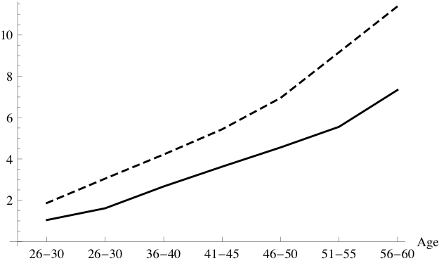
possible to an empirical measure of the same thing. Here, we choose to match the
median of the wealth to permanent income ratio across 7 age groups, from age
up to
.19
The choice of matching the medians rather the means is motivated by the fact that the wealth
distribution is much more concentrated at the top than the model is capable of
explaining using a single set of parameter values. This means that in practice one
must pick some portion of the population who one wants to match well; since the
model has little hope of capturing the behavior of Bill Gates, but might conceivably
match the behavior of Homer Simpson, we choose to match medians rather than
means.
As explained in section 3, it is convenient to work with the normalized version of the model
which can be written in Bellman form as:
with the first order condition:
(74)
(75)
The first substantive in this estimation procedure is to solve for the consumption functions
at each age. We need to discretize the shock distribution and solve for the policy functions by
backward induction using equation (75) following the procedure in sections 6 and ‘Recursion.’
The latter routine is slightly complicated by the fact that we are considering a life-cycle model
and therefore the growth rate of permanent income, the probability of death, the time-varying
discount factor and the distribution of shocks will be different across the years. We
thus must ensure that at each backward iteration the right parameter values are
used.
Correspondingly, the first part of the StructEstimation.py file begins by defining the agent
type by inheriting from the baseline agent type IndShockConsumerType, with the modification
to include time-varying discount factors. Next, an instance of this “life-cycle” consumer is
created for the estimation procedure. The number of periods for the life cycle of a given agent
is set and, following Cagetti, (?), we initialize the wealth to income ratio of agents at age
by randomly assigning the
equal probability values to ,
and
.
In particular, we consider a population of agents at age 25 and follow their
consumption and wealth accumulation dynamics as they reach the age of
, using
the appropriate age-specific consumption functions and the age-varying parameters. The
simulated medians are obtained by taking the medians of the wealth to income ratio of the
age
groups.
To complete the creation of the consumer type needed for the simulation, a history of shocks
is drawn for each agent across all periods by invoking the make_shock_history function. This
involves discretizing the shock distribution for as many points as the number of agents we
want to simulate and then randomly permuting this shock vector as many times as we need to
simulate the model for. In this way, we obtain a time varying shock for each agent. This is
much more time efficient than drawing at each time from the shock distribution a shock for
each agent, and also ensures a stable distribution of shocks across the simulation periods even
for a small number of agents. (Similarly, in order to speed up the process, at each backward
iteration we compute the consumption function and other variables as a vector at
once.)
With the age-varying consumption functions derived from the life-cycle agent, we can
proceed to generate simulated data and compute the corresponding medians. Estimating the
model involves comparing these simulated medians with empirical medians, measuring the
model’s success by calculating the difference between the two. However, before performing the
necessary steps of solving and simulating the model to generate simulated moments, it’s
important to note a difficulty in producing the target moments using the available
data.
Specifically, defining
as the set of parameters to be estimated (in the current case
), we
could search for the parameter values which solve
(76)
(77)
where
and are
respectively the empirical and simulated medians of the wealth to permanent income ratio for age
group .
A drawback of proceeding in this way is that it treats the empirically estimated medians as
though they reflected perfect measurements of the truth. Imagine, however, that
one of the age groups happened to have (in the consumer survey) four times as
many data observations as another age group; then we would expect the median to
be more precisely estimated for the age group with more observations; yet (77)
assigns equal importance to a deviation between the model and the data for all age
groups.
We can get around this problem (and a variety of others) by instead minimizing a slightly
more complex object:
(78)
(79)
where is the weight
of household in the
entire population,20
and
is the empirical wealth to permanent income ratio of household
whose head belongs
to age group .
is
needed because unequal weight is assigned to each observation in the Survey of Consumer
Finances (SCF). The absolute value is used since the formula is based on the fact that
the median is the value that minimizes the sum of the absolute deviations from
itself.
With this in mind, we turn our attention to the computation of the weighted median
wealth target moments for each age cohort using this data from the 2004 Survey of
Consumer Finances on household wealth. The objects necessary to accomplish this
task are weighted_median and get_targeted_moments. The actual data are taken
from several waves of the SCF and the medians and means for each age category
are plotted in figure 21. More details on the SCF data are included in appendix
A.
Figure 21: Wealth to Permanent Income Ratios from SCF (means (dashed) and medians
(solid))
We now turn our attention to the two key functions in this section of the code file. The first,
simulate_moments, executes the solving (solve) and simulation (simulation)
steps for the defined life-cycle agent. Subsequently, the function uses the agents’
tracked levels of wealth based on their optimal consumption behavior to compute
and store the simulated median wealth to income ratio for each age cohort. The
second function, smmObjectiveFxn, calls the simulate_moments function to create
the objective function described in (79), which is necessary to perform the SMM
estimation.
Thus, for a given pair of the parameters to be estimated, the single call to the function
smmObjectiveFxn executes the following:
solves for the consumption functions for the life-cycle agent
simulates the data and computes the simulated medians
We delegate the task of finding the coefficients that minimize the smmObjectiveFxn
function to the minimize_nelder_mead function, which is defined elsewhere and called in the
second part of this file. This task can be quite slow and rather problematic if the
smmObjectiveFxn function has very flat regions or sharp features. It is thus wise to verify the
accuracy of the solution, for example by experimenting with a variety of alternative starting
values for the parameter search.
The final object defined in this first part of the StructEstimation.py
file is calculateStandardErrorsByBootstrap. As the name suggests,
the purpose of this function is to compute the standard errors by
bootstrap.21
This involves:
drawing new shocks for the simulation
drawing a random sample (with replacement) of actual data from the SCF
obtaining new estimates for
and
We repeat the above procedure several times (Bootstrap) and take the standard deviation for
each of the estimated parameters across the various bootstrap iterations.
10.2.1 An Aside to Computing Sensitivity Measures
A common drawback in commonly used structural estimation procedures is a lack of
transparency in its estimates. As ? notes, a researcher employing such structural empirical
methods may be interested in how alternative assumptions (such as misspecification or
measurement bias in the data) would “change the moments of the data that the estimator uses
as inputs, and how changes in these moments affect the estimates.” The authors provide a
measure of sensitivity for given estimator that makes it easy to map the effects of different
assumptions on the moments into predictable bias in the estimates for non-linear
models.
In the language of ?, section 10 is aimed at providing an estimator
that has some true
value by assumption.
Under the assumption
of the researcher, the empirical targets computed from the SCF is measured
accurately. These moments of the data are precisely what determine our estimate
, which minimizes (79). Under
alternative assumptions ,
such that a given cohort is mismeasured in the survey, a different estimate is
computed. Using the plug-in estimate provided by the authors, we can see
quantitatively how our estimate changes under these alternative assumptions
which
correspond to mismeasurement in the median wealth to income ratio for a given age
cohort.
10.3 Results
The second part of the file StructEstimation.py defines a function main which produces our
and
estimates with standard errors using 10,000 simulated agents by setting the
positional arguments estimate_model and compute_standard_errors to
true.22
Results are
reported in Table 12.23
Table 11: Estimation Results
Table 12: Estimation Results
The literature on consumption and saving behavior over the lifecycle in the presence of labor income
uncertainty24
warns us to be careful in disentangling the effect of time preference and risk aversion when
describing the optimal behavior of households in this setting. Since the precautionary saving
motive dominates in the early stages of life, the coefficient of relative risk aversion (as well
as expected labor income growth) has a larger effect on optimal consumption and
saving behavior through their magnitude relative to the interest rate. Over time,
life-cycle considerations (such as saving for retirement) become more important and the
time preference factor plays a larger role in determining optimal behavior for this
cohort.
Using the positional argument compute_sensitivity, Figure 22 provides
a plot of the plug-in estimate of the sensitivity measure described in
10.2.1. As you can see from the figure the inverse relationship between
and
over the
life-cycle is retained by the sensitivity measure. Specifically, under the alternative assumption that
a particular cohort is mismeasured in the SCF dataset, we see that the y-axis suggests that our
estimate of
and
change in a predictable way.
Suppose that there are not enough observations of the oldest cohort of households in the
sample. Suppose further that the researcher predicts that adding more observations of these
households to correct this mismeasurement would correspond to a higher median wealth to
income ratio for this cohort. In this case, our estimate of the time preference factor should
increase: the behavior of these older households is driven by their time preference, so a higher
value of is
required to match the affected wealth to income targets under this alternative assumption.
Since risk aversion is less important in explaining the behavior of this cohort, a lower value of
is
required to match the affected empirical moments.
To recap, the sensitivity measure not only matches our intuition about the inverse relationship
between
and
over the life-cycle, but provides a quantitative estimate of what would happen to our estimates
of these parameters under the alternative assumption that the data is mismeasured in some
way.
Figure 22: Sensitivity of Estimates
regarding Alternative Mismeasurement Assumptions.
By setting the positional argument make_contour_plot to true, Figure 23 shows the
contour plot of the smmObjectiveFxn function and the parameter estimates. The contour plot
shows equally spaced isoquants of the smmObjectiveFxn function, i.e. the pairs of
and
which
lead to the same deviations between simulated and empirical medians (equivalent
values of equation (79)). Interestingly, there is a large rather flat region; or, more
formally speaking, there exists a broad set of parameter pairs which leads to similar
simulated wealth to income ratios. Intuitively, the flatter and larger is this region,
the harder it is for the structural estimation procedure to precisely identify the
parameters.
Figure 23: Contour Plot (larger values are shown lighter) with
Estimates (red dot).
11 Conclusion
Many choices can be made for solving microeconomic dynamic stochastic optimization
problems. The set of techniques, and associated code, described in these notes represents an
approach that I have found to be powerful, flexible, and efficient, but other problems may
require other techniques. For a much broader treatment of many of the issues considered here,
see Judd (?).
Appendices
A SCF Data
Data used in the estimation is constructed using the SCF 1992, 1995, 1998,
2001 and 2004 waves. The definition of wealth is net worth including housing
wealth, but excluding pensions and social securities. The data set contains
only households whose heads are aged 26-60 and excludes singles, following
Cagetti (?).25
Furthermore, the data set contains only households whose heads are college graduates. The
total sample size is 4,774.
In the waves between 1995 and 2004 of the SCF, levels of normal income are reported. The
question in the questionnaire is "About what would your income have been if it had been a normal
year?" We consider the level of normal income as corresponding to the model’s theoretical
object ,
permanent noncapital income. Levels of normal income are not reported in the 1992 wave.
Instead, in this wave there is a variable which reports whether the level of income is normal or
not. Regarding the 1992 wave, only observations which report that the level of income is
normal are used, and the levels of income of remaining observations in the 1992 wave are
interpreted as the levels of permanent income.
Normal income levels in the SCF are before-tax figures. These before-tax permanent income
figures must be rescaled so that the median of the rescaled permanent income of each age
group matches the median of each age group’s income which is assumed in the simulation.
This rescaled permanent income is interpreted as after-tax permanent income. Rescaling is
crucial since in the estimation empirical profiles are matched with simulated ones which are
generated using after-tax permanent income (remember the income process assumed in the
main text). Wealth / permanent income ratio is computed by dividing the level of
wealth by the level of (after-tax) permanent income, and this ratio is used for the
estimation.26